One of my favorite sabermetric baseball articles of all time was written by Sky Andrecheck in 2010 — part as a meditation on the purpose/meaning of playoffs, and part as a solution for some of the thorny logical concerns that arise from said mediation.

The basic conundrum for Andrecheck revolved around the very existence of a postseason tournament, since — logically speaking — such a thing should really only be invoked to resolve confusion over who the best team was during the regular season. To use a baseball example, if the Yankees win 114 games and no other AL team wins more than 92, we can say with near 100% certainty that the Yankees were the AL’s best team. There were 162 games’ worth of evidence; why make them then play the Rangers and Indians on top of that in order to confirm them as the AL’s representative in the World Series?

Andrecheck’s solution to this issue was to set each team’s pre-series odds equal to the difference in implied true talent between the teams from their regular-season records. If the Yankees have, say, a 98.6% probability of being better than the Indians from their respective regular-season records, then the ALCS should be structured such that New York has a 98.6% probability of winning the series — or at least close to it (spot the Yankees a 3-0 series lead and every home game from that point onward, and they have a 98.2% probability of winning, which is close enough). [continue reading…]

The Simple Rating System is a many-splendored thing, but a known bug of the process is that huge outlier scoring margins can have undue influence on the rankings. Take the 2009 NFL season, for instance, during which the Patriots led the NFL in SRS in no small part because they annihilated the Titans 59-0 in a snowy October game that tied for the second-most lopsided margin of victory in NFL history. Outside of that single game, the Patriots’ PPG margin was +5.2, which wouldn’t have even ranked among the league’s top ten teams, but the SRS (particularly because it minimizes squared prediction errors between actual outcomes and those expected from team ratings) gave the 59-0 win a lot of weight, enough to propel New England to the #1 ranking. (A placement that looked downright laughable, I might add, when the Pats were crushed at home by Baltimore on Wild Card Weekend.)

One solution that is commonly proposed for this problem is to cap the margin of victory in a given game at a certain fixed number. This is especially popular in college football (in fact, Chase sort of uses a cap in his college SRS variant) because nonconference schedules will often see matchups between teams of incredibly disparate talent levels, games in which the powerhouse team can essentially choose the margin by which they want to steamroll their opponent. Within that context, it doesn’t really matter whether Florida State beats Idaho by 46 or by 66, because there’s a 0% chance Idaho is a better team than FSU — no new information is conveyed when they pile more and more points onto the game’s margin.

But what’s the right number to cap margin of victory at in the NFL? These are all professional teams, after all, so there’s plenty of evidence that in the NFL, blowing opponents out — even when they’re bad teams — says a lot about how good you are. Where do we draw the line, then, to find the point at which a team has clearly proven they’re better than the opponent, beyond which any extra MOV stops giving us information?

[continue reading…]

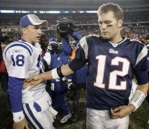
Presented below, without comment, is a table of every matchup featuring Tom Brady & Peyton Manning as the starting quarterbacks. Enjoy:

(I originally posted this at the S-R Blog, but I thought it would be very appropriate here as well.)

Just a quick hit of a post to let you know that tonight’s MNF matchup between the 0-6 Giants and the 1-4 Vikings is, in fact, the worst ever this late in the season by combined winning percentage:

It is not, however, the worst by combined PPG margin. That honor belongs to this 1972 game between the 2-5 Patriots and the 1-6 Colts (Baltimore ended up winning 24-17):

Last week, we announced that our True Receiving Yards metric has now been calculated back to 1950, so it’s only fitting that we also compute WOWY (With Or Without You) for all of those receivers as well.

Skip the paragraph after this if you don’t care about the gory mathematical details, and just know that WOWY basically answers the question: “Did a receiver’s quarterbacks play better when they threw a lot to him, or not?”

For the brave souls who care about the calculation: WOWY starts by measuring the difference between a QB’s age-adjusted Relative Adjusted Net Yards Per Attempt in a given season and his combined age-adjusted RANY/A in every other season of his career. This is computed as an average for each team’s QB corps, using a combination of QB dropbacks during the season in question and the rest of his career as the weights (the exact formula is: weight = 1/(1/drpbk_year + 1/drpbk_other)). Finally, for each receiver we compute a weighted career average of the QB WOWY scores for the teams he played on, weighted by his True Receiving Yards in each season.

At any rate, the only players who don’t get a WOWY are those who either debuted before 1950, played with a QB who debuted before 1950, or played with a QB who ever threw to a receiver who debuted before 1950. Here are the career WOWY marks (when applicable), alongside TRY, for every 3,000-TRY receiver whose career started in 1950 or later:

[continue reading…]

As Jason Lisk and I wrote about before the season, Tom Brady and Ben Roethlisberger have become something of the poster children so far this year when it comes to veteran QBs working with inexperienced and otherwise less-than-notable receiving groups. And, lo and behold, each has put up career-low RANY/A marks through 2 games. But how do their receiving corps rank relative to those of other teams so far this year, and how do they stack up historically?

To take a stab at answering these questions, I turned to True Receiving Yards. For each player who debuted in 1950 or later, I computed their Weighted Career True Receiving Yards for every year, as of the previous season, to get a sense of how experienced/accomplished they’d been going into the season in question. Then, I calculated a weighted averaged of those numbers for every receiver on a given team, using TRY during the season in question as the weights. For example, here are the 2013 Patriots receivers:

The way to read that is: Julian Edelman has accounted for 38 percent of the Pats’ TRY so far. Going into the season, he had a career Weighted TRY of 615.7, so he contributes to 38% of the 2013 Pats’ weighted average with his 615.7 previous career weighted TRY; Danny Amendola contributes to 20% of the team weighted average with his 1541.9 previous career weighted TRY; etc. Multiply each guy’s previous weighted career TRYs by the percentage of the team’s 2013 TRY he contributed, and you get a cumulative weighted average of 560.7 — meaning the average TRY of a 2013 Pats receiver has been gained by a guy who had a previous career weighted TRY of 560.7.

Is that a low number? Well, here are the numbers for all of the 2013 team receiving corps (not including Thursday night’s Eagles-Chiefs tilt), inversely sorted by weighted average (asterisks indicate rookies):

[continue reading…]

About a month ago, Chase & I developed a stat called True Receiving Yards, which seeks to put all modern & historical receiving seasons on equal footing by adjusting for the league’s passing YPG environment & schedule length, plus the amount the player’s team passed (it’s easier to produce raw receiving stats on a team that throws a lot), with bonuses thrown in for touchdowns and receptions. It’s not perfect — what single stat in a sport with so many moving parts is? — but it does a pretty good job of measuring receiving productivity across different seasons and across teams with passing games that operated at vastly different volumes.

Anyway, today’s post is basically a data dump to let everyone know we’ve extended TRY data back to 1950 (before, it was only computed for post-merger seasons). Here are the new all-time career leaders among players who debuted in 1950 or later (see below for a key to the column abbreviations):
[continue reading…]

In 1998, 21-year-old Randy Moss made a stunning NFL debut, racking up 17 touchdowns and 1,260 True Receiving Yards, the 2nd-best total in football that season. The Vikings’ primary quarterback that year, Randall Cunningham, was a former Pro Bowler and MVP, but all that seemed like a lifetime ago before the ’98 season. He’d been out of football entirely in 1996, and in 1997 he posted an Adjusted Net Yards per Attempt average that was 1.2 points below the league’s average (for reference’s sake, replacement level is usually around 0.75 below average). With Moss in ’98, though, Cunningham’s passing efficiency numbers exploded: he posted a career best +3.2 Relative Adjusted Net Yards per Attempt, miles ahead of his perfectly-average overall career mark. If we adjust for the fact that Cunningham was also 35 at the time (an age at which quarterbacks’ RANY/A rates tend to be 1.1 points below what they are at age 27), Cunningham’s 1998 rate was actually 4.3 points better than we’d expect from the rest of his career, a staggering outlier.

The following year, Jeff George took over as the Vikings primary quarterback, and he promptly posted a Relative ANY/A 2.2 points higher than expected based on his age and the rest of his career. ^[1]Cunningham’s RANY/A was also 1.0 better than expected in limited action. George left Moss and Minnesota after the season, and he would throw only 236 passes the rest of his career, producing a cumulative -0.6 RANY/A in Washington before retiring.

From 2000-04, Moss was the primary target of Daunte Culpepper, whose RANY/A was 0.7 better than expected (based on Culpepper’s career numbers) when Moss was around. ^[2]That number is an average weighted by the number of TRY Moss had in each season Although he’d enjoyed one of the best quarterback seasons in NFL history in 2004, Culpepper was never the same after Moss was traded to Oakland; in fact, he never even had another league-average passing season, producing a horrible -1.2 RANY/A from 2005 until his retirement in 2009. ^[3]To be fair, Culpepper tore his ACL, MCL, and PCL halfway through the 2005 season, which also was a factor in his decline.

Moss’s stint with the Raiders was famously checkered — although Kerry Collins’ RANY/A was 0.6 better than expected in 2005, Aaron Brooks played 2.5 points of RANY/A below his previous standards in 2006 — but we all know what happened when he joined the Patriots in 2007. With Moss, Tom Brady’s RANY/A was a whopping 1.3 points higher than expected from the rest of his career, and Moss also played a big role in Matt Cassel’s RANY/A being +1.0 relative to expectations after Brady was lost for the season in 2008.

While Moss’s post-Pats career hasn’t exactly been the stuff of legends, the majority of his career (weighted by True Receiving Yards) saw him dramatically improve his quarterbacks’ play relative to the rest of their careers. In fact, his lifetime WOWY (With or Without You) mark of +1.1 age-adjusted RANY/A ranks 3rd among all receivers who: a) had at least 3,000 career TRY, b) started their careers after the merger, and c) played exclusively with quarterbacks who started their careers after the merger. And the first two names on the list are possibly explained by other means. The table below lists all 301 receivers with 3,000 career TRY. The table is fully sortable and searchable, and you can click on the arrows at the bottom of the table to scroll. The table is sorted by the QB WOWY column.
[continue reading…]

While the state of the Steelers’ receiving corps isn’t as shaky as say, that of the New England Patriots, it could certainly be called an area of potential concern for Ben Roethlisberger and the Pittsburgh offense going into 2013. One of the biggest moves on the first day of free agency involved Mike Wallace departing for Miami; meanwhile, Heath Miller’s injury status — while more encouraging than previously thought — will cost him several games, and probably some effectiveness when he does eventually return. All of this comes on the heels of losing stealth HoFer Hines Ward (albeit an older, drastically less effective version) to retirement after the 2011 season.

For Roethlisberger, this downturn in the quality of his receivers is a pretty new phenomenon. In fact, by one measure of career receiving-corps talent (which I’ll explain below), Big Ben has been blessed with the fourth-most gifted receiving group among current starting quarterbacks with more than two years of experience (behind only Peyton Manning, Matt Ryan, and Tony Romo). In fact, Roethlisberger’s 16th-ranked receiving corps in 2012 was by far the least talented group of pass catchers he’s ever had to throw to.

How do you begin to measure the quality of a quarterback’s receiving corps, you ask? Well, pretty much any method is going to fraught with circular logic, especially if a quarterback consistently has the same receivers over several years. His successes are theirs, and vice-versa. However, here’s one stab at shedding at least some light on the issue.

For each team since the NFL-AFL merger, I:

• Gathered all players with at least 1 catch for the team in the season.
• Computed their True Receiving Yards in that season; I then determined what percentage of the team’s True Receiving Yards was accumulated by which receiver in each year. For example, Hines Ward had 1,029 TRY in 2009, which represented 25.9% of the 3,979 True Receiving Yards accumulated by all Steelers that year
• Figured out the most TRY they ever had in a season, a number I’m calling each player’s peak TRY; for Ward, his peak TRY is equal to 1,279.
• Calculated a weighted average (based on the percentage of team TRY gained by each receiver) of the receivers’ peak TRY (weighted by their TRY during the season in question).

(I also threw out all teams that had a receiver who debuted before 1970, since I don’t know what the real peak TRY of any pre-merger receiver was. I should eventually calculate TRY for pre-merger seasons, of course — thank you Chase & Don Maynard.)

As an example, here are the 2009 Steelers, the most talented corps of receivers Roethlisberger has had in his career:
[continue reading…]

More than a decade ago (on a side note: how is that possible?), Doug wrote a series of player comments highlighting specific topics as they related to the upcoming fantasy football season. I recommend that you read all of them, if for no other reason than the fact you should make it a policy to read everything Doug Drinen ever wrote about football, but today we’re going to focus on the Isaac Bruce comment, which asked/answered the question:

Is this Ram team the biggest fantasy juggernaut of all time?

“This Ram team,” of course, being the 1999, 2000, & 2001 Greatest Show on Turf St. Louis Rams. At the time, Doug determined that those Rams were not, in fact, the best real-life fantasy team ever assembled, by adding up the collective VBD for the entire roster. They ranked tenth since 1970; the top 10 were:

1. 1. 1975 Buffalo Bills – 550 Simpson (281) Ferguson (98) Braxton (83) Chandler (44) Hill (42)

2. 1982 San Diego Chargers – 542 Chandler (190) Fouts (126) Winslow (121) Muncie (92) Brooks (10) Joiner (1)

3. 1994 San Francisco 49ers – 514 Young (208) Rice (140) Watters (98) Jones (67)

4. 1995 Detroit Lions – 478 Mitchell (136) Moore (132) Sanders (121) Perriman (87)

5. 1984 Miami Dolphins – 470 Marino (243) Clayton (145) Duper (76) Nathan (6)

6. 1998 San Francisco 49ers – 467 Young (200) Hearst (137) Owens (81) Rice (46) Stokes (1)

7. 1986 Miami Dolphins – 456 Marino (210) Duper (94) Clayton (76) Hampton (61) Hardy (13)

8. 2000 Minnesota Vikings – 452 Culpepper (170) Moss (123) Smith (87) Carter (70)

9. 1991 Buffalo Bills – 449 Thomas (157) Kelly (143) Reed (80) Lofton (51) McKeller (17)

10. 1999 St. Louis Rams – 435 Faulk (184) Warner (179) Bruce (71)

As an extension of Chase’s recent post on the The Best Skill Position Groups Ever, we thought it might be useful to update Doug’s study in a weekend data-dump post. I modified the methodology a bit — instead of adding up VBD for the entire roster, for each team-season I isolated the team’s leading QB and top 5 non-QBs by fantasy points (using the same point system I employed when ranking the Biggest Fluke Fantasy Seasons Ever). I then added up the total VBD of just those players, to better treat each roster like it was a “real” fantasy team.

Anyway, here are the results. Remember as well that VBD is scaled up to a 16-game season, so as not to short-change dominant fantasy groups from strike-shortened seasons (:cough:1982 Chargers:cough:).
[continue reading…]

Yesterday, I set up a method for ranking the flukiest fantasy football seasons since the NFL-AFL merger, finding players who had elite fantasy seasons that were completely out of step with the rest of their careers. I highlighted fluke years #21-30, so here’s a recap of the rankings thus far:

30. Lorenzo White, 1992
29. Dwight Clark, 1982
28. Willie Parker, 2006
27. Lynn Dickey, 1983
26. Robert Brooks, 1995
25. Ricky Williams, 2002
24. Jamal Lewis, 2003
23. Mark Brunell, 1996
22. Vinny Testaverde, 1996
21. Garrison Hearst, 1998

Now, let’s get to…

The Top Twenty

20. RB Natrone Means, 1994

Best Season
year	g	rush	rushyd	rushtd	rec	recyd	rectd	VBD
1994	16	343	1,350	12	39	235	0	103.0
2nd-Best Season
year	g	rush	rushyd	rushtd	rec	recyd	rectd	VBD
1997	14	244	823	9	15	104	0	12.9

Big, bruising Natrone Means burst onto the scene in 1994 as a newly-minted starter for the Chargers’ eventual Super Bowl team, gaining 1,350 yards on the ground with 12 TDs. In the pantheon of massive backs, he was supposed to be the AFC’s answer to the Rams’ Jerome Bettis, but Means was slowed by a groin injury the following year and never really stayed healthy enough to recapture his old form. The best he could do was to post a pair of 800-yard rushing campaigns for the Jaguars & Chargers in 1997 & ’98 before retiring after the ’99 season.

19. WR Braylon Edwards, 2007

Best Season
year	g	rec	recyd	rectd	VBD
2007	16	80	1,289	16	107.7
2nd-Best Season
year	g	rec	recyd	rectd	VBD
2010	16	53	904	7	15.4

The 3rd overall pick in the 2005 Draft out of Michigan, Edwards seemingly had a breakout 2007 season catching passes from fellow Pro Bowler Derek Anderson. But both dropped off significantly the next season, and Edwards was sent packing to the Jets in 2009. He did post 904 yards as a legit starting fantasy wideout in 2010, but he has just 380 receiving yards over the past 2 seasons, and it’s not clear he’ll ever live up to those eye-popping 2007 numbers again.
[continue reading…]

There’s nothing like a truly great fluke fantasy season. Because they can help carry you to a league championship (and therefore eternal bragging rights — flags fly forever, after all), a random player who unexpectedly has a great season will often have a special place in the heart of every winning owner. And even if you only use their jerseys as makeshift aprons to cook in, fluke fantasy greats are a part of the fabric of football fandom. That’s why this post is a tribute to the greatest, most bizarre, fluke fantasy seasons of all time (or at least since the 1970 NFL-AFL merger).

First, a bit about the methodology. I’m going to use a very basic fantasy scoring system for the purposes of this post:

• 1 point for every 20 passing yards
• 1 point for every 10 rushing or receiving yards
• 6 points for every rushing or receiving TD
• 4 points for every passing TD
• -2 points for every passing INT

I’m also measuring players based on Value Based Drafting (VBD) points rather than raw points. In a nutshell, VBD measures true fantasy value by comparing a player to replacement level, defined here as the number of fantasy points scored by the least valuable starter in your league. For the purposes of this exercise, I’m basing VBD on a 12-team league with a starting lineup of one QB, two RBs, 2.5 WRs, and 1 TE. That means we’re comparing a player at a given position to the #12-ranked QB, the #24 RB, the #30 WR, or the #12 TE in each season. If a player’s VBD is below the replacement threshold at his position, he simply gets a VBD of zero for the year.
[continue reading…]

Back in March, Chase wrote a post investigating how quarterbacks age, finding that they peak at age 29 (with a generalized peak from 26-30) in terms of value over average. Today, I thought I’d quickly look at how quarterbacks age in terms of their performance rate — specifically, their Adjusted Net Yards per Attempt (ANY/A). For newer readers, ANY/A is based on the following formula: (Passing Yards + 20 * Passing TDs – 45 * INTs – Sack Yards Lost) / (Pass Attempts + Sacks).

First, I need to introduce a way of adjusting ANY/A for era: Relative ANY/A. Relative ANY/A is simply equal to:

QB_ANY/A – LgAvg_ANY/A

The table below lists the 30 single-season leaders in Relative ANY/A since the merger. You won’t be too surprised to see the 2004 version of Peyton Manning at the top. That year, Manning averaged 9.8 ANY/A, while the league average was just 5.6 ANY/A. That means Manning gets a Relative ANY/A grade of +4.1 (with the difference due to rounding).
[continue reading…]

(I originally posted this at the S-R Blog, but I thought it would be very appropriate here as well.)

Here is a google doc containing every team-season in our database since 1957, including the Head Coach and offensive & defensive coordinators. It also specifies those coaches’ preferred offensive or defensive schemes (depending on which side of the ball they specialize in), and attempts to figure out the general offensive family (i.e. Air Coryell, Erhardt-Perkins, etc) each team-season fell into.

THIS IS BY NO MEANS COMPLETE. In fact, it’s very much incomplete at this stage — and that’s where you come in. In the comments of this post, or in an email, we’d love to hear corrections and/or additions to the data, if you see an entry about which you know more than we do (and it’s a good bet you do). Thanks in advance for your help, and hopefully we can assemble a more complete listing of teams’ systems/schemes, which will let us do things like compute splits vs. a certain type of offense or defense, analyze whether 4-3 or 3-4 defenses were better in a given season, etc.

So let those corrections/additions pour in!

Last week, Chase had a great post where he looked at what percentage of the points scored by a team in any given game is a function of the team, and what percentage is a function of the opponent. The answer, according to Chase’s method, was 58 percent for the offense and 42 percent for the defense (note that, in the context of posts like these, “offense” means “scoring ability, including defensive & special-teams scores”, and “defense” means “the ability to prevent the opponent from scoring”). Today I’m going to use a handy R extension to look at Chase’s question from a slightly different perspective, and see if it corroborates what he found.

My premise begins with every regular-season game played in the NFL since 1978. Why 1978? I’d love to tell you it was because that was the year the modern game truly emerged thanks to the liberalization of passing rules (which, incidentally, is true), but really it was because that was the most convenient dataset I had on hand with which to run this kind of study. Anyway, I took all of those games, and specifically focused on the number of points scored by each team in each game. I also came armed with offensive and defensive team SRS ratings for every season, which give me a good sense of the quality of both the team’s offense and their opponent’s defense in any given matchup.

If you know anything about me, you probably guessed that I want to run a regression here. My dependent variable is going to be the number of points scored by a team in a game, but I can’t just use raw SRS ratings as the independent variables. I need to add them to the league’s average number of points per game during the season in question to account for changing league PPG conditions, lest I falsely attribute some of the variation in scoring to the wrong side of the ball simply due to a change in scoring environment. This means for a given game, I now have the actual number points scored by a team, the number of points they’d be expected to score against an average team according to SRS, and the number of points their opponents would be expected to allow vs. an average team according to SRS.
[continue reading…]

Now that we live in a world where Joe Flacco and Eli Manning have quarterbacked 3 of the last 6 Super Bowl-winning teams, you might be tempted to think that winning a Super Bowl as a QB doesn’t mean what it used to. After all, the playoffs are getting more random — as Aaron Schatz pointed out last night, four of the last six Super Bowl champs have finished the regular season with 10 or fewer wins. So it stands to reason that, as the championship teams themselves post less-remarkable seasons, so too would their quarterbacks not be the cream of the crop. And for all of his postseason brilliance, Flacco was just the league’s 17th-best quarterback during the regular season. Does his ascendancy, coming on the heels of Manning’s, signal a new trend?

To answer that question, I turned to a methodology I’ve used many times before. The basic premise is that, to put modern and historical quarterbacks on an even playing field (no pun intended), you must translate their stats into a common environment. To do this, you take the quarterback’s stats from a given season, pro-rate to 16 scheduled games, and multiply by the ratio of the league’s per-game average during the season in question to that of a common reference season. For instance, if I’m adjusting Terry Bradshaw’s 1977 passing yards to the 1991-2012 period, I would multiply his actual total of 2,523 by (16/14) to account for the shorter season that year, then multiply that by (225.1/162.2) to account for the change in the league’s passing environment, giving an adjusted total of 4,001 yards.

After doing that for every QB season since the merger, I then plugged the translated stats into a regression formula that predicts Football Outsiders’ Yards Above Replacement based on the QB’s box score stats (including the standard cmp/att/yds/td/int, plus sacks, fumbles, and rushing stats). This gives us Estimated Yards Above Replacement (eYAR) a measure of total value for each QB season, adjusted for schedule length and league passing conditions, which is perfect for historical analysis.

To get an idea of what we’re talking about, here are Flacco’s career translated stats and eYAR numbers:
[continue reading…]

Eight years ago — almost to the day — our old PFR colleague Doug Drinen wrote a Sabernomics post about “The Manning Index”, a metric designed to roughly gauge the clutchness (or chokeitude) of a given quarterback by looking at how he did relative to expectations (he revived this concept in version two, six years ago). In a nutshell, Doug used the location of the game and the win differential of the two teams involved to establish an expected winning percentage for each quarterback in a given matchup. He then added those up across all of a quarterback’s playoff starts, and compared to the number of wins he actually had. Therefore, quarterbacks who frequently exceeded expectations in playoff games could be considered “clutch” while those who often fell short (like the Index’s namesake, Peyton Manning) might just be inveterate chokers.

Doug ran that study in the midst of the 2004-05 playoffs, so it shouldn’t be surprising that Tom Brady (who was at the time 8-0 as a playoff starter and would run it to 10-0 before ever suffering a loss) came out on top, winning 3.5 more games than you’d expect from the particulars of the games he started. Fast-forward eight years, though, and you get this list of quarterbacks who debuted after 1977:
[continue reading…]

Presented without comment, the most current Simple Ratings, weighted for recency:

“Upper” and “Lower” are the 95% confidence intervals around each estimate. Roughly speaking, this means we can be 95% confident that, say, the 49ers’ “true” SRS rating is between 3.66 and 16.80.

This is mostly a huge end-of-regular-season data dump, but I’ll explain a little before the table…

PFR’s Simple Rating System can be broken into offensive and defensive components, which represent the number of points per game the team scored/allowed per game compared to the league average, after adjusting for the strength of opposing offenses and defenses faced. If you want to derive an expected winning percentage from that, you have to “back out” to total points scored/allowed again. To do that, you just add OSRS (or subtract DSRS) to the league’s average PPG, then multiply by the number of games the team played. This will give you adjusted points scored/allowed totals for the season.

To get that into a winning percentage-like form, you then need to plug those totals into the Pythagorean Formula. It usually takes the form of

(Pts Scored ^ x) / (Pts Scored ^ x + Pts Allowed ^ x)

where x was determined to be around 2.4 for the NFL in the 1990s, when current Houston Rockets (yep, basketball) GM Daryl Morey researched it for STATS, Inc. Last year, Football Outsiders decided to employ a “floating” exponent that varies with the scoring environment in which a team played, recognizing that a single point is more important to winning in lower-scoring environments. To that end, they used what’s known as the “Pythagenport” method of determining the exponent, which is

1.5 * log10((PF + PA) / G)

I was poking around in the data the other day, though, and found that the so-called “Pythagenpat” variant actually correlates slightly better with teams’ actual won-lost records since the NFL-AFL merger. That formula suggests for each team an exponent of

((PF + PA) / G) ^ 0.2466

This gives you a 1.204 RMSE vs. wins since 1970, a very slight improvement over the 1.205 RMSE you get using FO’s formula.

At any rate, I applied the Pythagenpat exponent to each team’s schedule-adjusted points scored/allowed totals since 1970, and tweaked the pythagorean win/loss totals up/down at the league-season level to match actual league-wide win/loss totals. The result was a definitive set of pythagorean ratings for every team since the merger:

Now, as an aside, I wouldn’t go plugging those directly into the log5 formula to predict this weekend’s games just yet. You first need to regress to the mean to account for the uncertainty we see in any observed result. To do that, just add about 17.65 games of .500 performance to each team’s pythagorean Wpct, and you’ll get a “true talent” number that should yield more accurate probabilities regarding future outcomes.

I’ve been on a major QB kick lately, and there’s no reason to stop now. Today, I want to look at a method that might tease out a quarterback’s “true talent” better than if we simply use his raw stats from the season.

Three years ago, our colleague Jason Lisk had a post on the old PFR Blog about which rate stats stay consistent when a QB changes teams. Basically, he grabbed QBs who were still in their primes and changed teams, looking at how their key rate stats correlated from one year to the next. Here’s what Jason found:

[…]I looked at the correlation coefficient for our group of 48 passers, for the year N advanced passing score compared to the year N+1 advanced passing score in each category. This should tell us whether the passers who were good in a performance area (or bad) tended to be the ones who remained good in that performance area the following season, even with the uncertainty of team changes (some positive, some negative for the quarterback).

Sack Percentage:  0.31
Completion Percentage: 0.25
Yards Per Attempt:  0.20
Touchdown Percentage: 0.12
Interception Percentage: 0.10

What do those correlations mean, exactly? Well, take sack percentage as an example. In general, a correlation of 0.31 means you can expect 31% of a QB’s difference from the mean to be repeated next year when he changes teams. In other words, you have to regress the QB’s sack rate 69% towards the mean to get the true rate that “belongs” to him. If the average sack rate is 6.1%, and a QB has a rate of 4.0% (like, say, Drew Brees this year), his “true” sack rate is probably something like 5.4% — 31% of the distance between .061 and .040.

The same concept applies to the other stats listed above. Tony Romo’s observed 66.7% completion percentage is really more like 62.5% after regressing to the mean, and so forth. Do that for every QB who had a reasonable number of attempts this year, and you get these rate stats:

(“A-” before a stat means the actual observed rate; “R-” means the regressed rate.)

Now we just need to reconstruct the player’s raw passing line as though he posted those rate stats instead of his actual rates. Cmp%, YPA, TD%, and INT% are easy (just multiply by attempts), and Sack% can be derived via simple algebra:

Sacks_new = (-reg_sk% * Attempts) / (reg_sk% – 1)

(Sack yards can be assumed by multiplying raw sack yards per sack by the new sack total.)

Finally, we plug the new totals into the Adjusted Net Yards Per Attempt formula, and we have a QB stat that is sort of like baseball’s Fielding Independent Pitching (FIP), which also seeks to reduce the noise and teammate interactions in a pitcher’s ERA by reducing his performance to only those elements he has control over — strikeouts, walks, and home runs.

Here are the 2012 leaders in QB-FIP (along with their regressed totals):

After posting about SRS-style quarterback ratings on Monday, I was thinking about other things we can do with game-by-game data like that. In his QBGOAT series, Chase likes to compare QBs to the league average, which makes a lot of sense for all-time ratings — you want to reward guys who are at least above-average in a ranking like that. However, if we want seasonal value, perhaps average is too high a baseline.

Over at Football Outsiders, Aaron Schatz has always compared to “replacement level”, borrowing a concept from baseball. I like that approach, but replacement level can be hard to empirically determine. So for the purposes of this post, I wanted to come up with a quick-and-dirty baseline to which we can compare QBs.

To that end, I looked at all players who were not their team’s primary passer in each game since 2010. Weighted by recency and the number of dropbacks by each passer, they performed at roughly a 4.4 Adjusted Net Yards Per Attempt level. This is not necessarily the replacement level, but it does seem to be the “bench level” — i.e., the ANYPA you could expect from a backup-caliber QB across the league.

Using 4.4 ANYPA as the baseline, we get the following values for 2012:

If we weigh each game by how recent the results took place, we get this list:

This kind of thing isn’t exactly the most advanced stat in the world, but it’s pretty good if you want to sort QBs into general groups based on how good they are (the assumption being that a player who never plays is implicitly a bench-level player by definition).

Here’s a quick set of quarterback ratings I was messing around with, based on Doug’s Simple Rating System. The basic setup: I took every passer-game (Att > 0) since the 2010 season, weighting for recency according to Wayne Winston’s method. I ran the data through the SRS to adjust for the quality of opponent pass defenses, creating a predicted Net YPA rate for each passer in each game via the following formula:

Predicted NYPA = League Constant + Home-Field Advantage + Passer Rating – Opponent Pass D Rating

The league constant in this case was a Net YPA of 6.24; the homefield component (which was positive while at home, negative on the road, and 0 in Super Bowls) was 0.05. Minimize the sum of squared errors between predicted and actual NYPA for each passer-game (weighted by recency and how many dropbacks the passer had in the game), and you’ve got a set of opponent-adjusted, recency-weighted QB ratings.

Throwing out the Brett Favres and Curtis Painters of the world who haven’t been active this year, here are the full ratings:

[continue reading…]

On November 15, 2010, Michael Vick humiliated the Washington Redskins before a national television audience on Monday Night Football. The big news right before kickoff was that the ‘Skins had signed former Eagle QB Donovan McNabb to a five-year, $78 million contract extension, an ironic note that wouldn’t be lost on observers as McNabb’s replacement, Vick, put together one of the greatest all-around quarterbacking performances in NFL history:

McNabb, on the other hand, was mediocre, going 17-31 with 295 yards and 2 TDs, but also 3 picks. More damning, Washington’s offense produced zero points until the Redskins were in a 35-0 hole and the game was essentially over.

Fast-forward 735 days, though, and the Redskins got their payback. An injured Vick was on the shelf, the Eagles entered the game on a 5-game losing streak, and electrifying rookie Robert Griffin III extended it to six with a brilliant performance of his own:

So, which performance was better, Vick’s original or RGIII’s remix? Vick threw for 133 more yards, rushed for practically the same amount as Griffin (on 4 fewer carries), and produced more total TDs. Then again, Griffin completed 93% of his passes and put together the vaunted 158.3 “perfect” QB rating. It’s a tough call.

Sound off with your opinion below!

Here’s my weekly set of power ratings, according to a weighted version of the Simple Rating System:

KEY:
Talent – Regressed WPct talent for 2012; Talent = (W + 5.5) / (G + 11)
PWAG – Probability of Winning Any Game
Off – Offensive SRS (positive = better)
Def – Defensive SRS (negative = better)
SRS – Simple Rating System (Off + Def)
wpa_loc – Win Probability Added from location of games
wpa_veg – Win Probability Added from Vegas lines
wpa_1st – Win Probability Added in 1st quarter
wpa_2nd – Win Probability Added in 2nd quarter
wpa_3rd – Win Probability Added in 3rd quarter
wpa_4ot – Win Probability Added in 4th qtr/overtime

In Tuesday’s post, I outlined a method of regressing a team’s record to the mean to estimate its “true winning percentage talent” (the trick is to add eleven games of .500 ball to their record, at any point in the season). In the comments, FP reader Dave wondered if we could incorporate last year’s true WPct talent into our talent assessment for this season, so I thought I’d run a quick regression to look at that.

My dataset was simply every game from 2003-2012 (including Monday night’s game). For each game, I recorded:

• Whether the game was a win, loss, or tie for the team in question. Wins got you a “1”, ties a “0.5”, losses a “0”.
• The team’s WPct talent estimate going into the game. So in the first game of the season, that’s (0+5.5)/(0+11)=0.500 for everybody; meanwhile, for an 11-4 team going into the final game of the season, it’s (11+5.5)/(15+11)=0.635.
• The team’s WPct talent estimate from the previous season.

I then set up a logistic regression to predict whether the game was a win or a loss based on the two WPct talent variables, this year and last year:

Deviance Residuals: 
    Min       1Q   Median       3Q      Max  
-1.7686  -1.1489   0.1616   1.1429   1.7072  

Coefficients:
              Estimate Std. Error z value Pr(>|z|)    
(Intercept)    -2.6936     0.1982 -13.589  < 2e-16 ***
currenttalent   4.0297     0.3509  11.485  < 2e-16 ***
prevtalent      1.3571     0.2666   5.091 3.57e-07 ***
---
Signif. codes:  0 ‘***’ 0.001 ‘**’ 0.01 ‘*’ 0.05 ‘.’ 0.1 ‘ ’ 1 

(Dispersion parameter for binomial family taken to be 1)

    Null deviance: 6712.4  on 4843  degrees of freedom
Residual deviance: 6508.0  on 4841  degrees of freedom
AIC: 6516.1

Number of Fisher Scoring iterations: 4

That means to predict your likelihood of winning any given game, you plug your WPct talent numbers from this season and last season into this formula:

WPct ~ 1 / (1 + EXP(2.693606 - 4.029688*(Current_Talent) - 1.357123*(Prev_Talent)))

It's important to note the size of the coefficients here -- the current WPct talent coefficient is three times as big as that of last season's WPct talent, so it has much more bearing on the prediction.

At any rate, here are the probabilities of winning any given game that this formula implies for this year's teams:

(I originally posted this at the S-R Blog, but I thought it would be very appropriate here as well.)

WARNING: Math post.

PFR user Brad emailed over the weekend with an interesting question:

“Wondering if you’ve ever tracked or how it would be possible to find records vs. records statistics….for instance a 3-4 team vs. a 5-2 team…which record wins how often? but for every record matchup in every week.”

That’s a cool concept, and one that I could answer historically with a query when I get the time. But in the meantime, here’s what I believe is a valid way to estimate that probability…

1. Add eleven games of .500 ball to the team’s current record (at any point in the season). So if a team is 3-4, their “true” wpct talent is (3 + 5.5) / (7 + 11) = .472. If their opponent is 5-2, it would be (5 + 5.5) / (7 + 11) = .583.
2. Use the following equation to estimate the probability of Team A beating Team B at a neutral site:
   

   p(Team A Win) = Team A true_win% *(1 – Team B true_win%)/(Team A true_win% * (1 – Team B true_win%) + (1 – Team A true_win%) * Team B true_win%)

3. You can even factor in home-field advantage like so:
   

   p (Team A Win) = [(Team A true_win%) * (1 – Team B true_win%) * HFA]/[(Team A true_win%) * (1 – Team B true_win%) * HFA +(1 – Team A true_win%) * (Team B true_win%) * (1 – HFA)]

   In the NFL, home teams win roughly 57% of the time, so HFA = 0.57.

This means in Brad’s hypothetical matchup of a 5-2 team vs. a 3-4 team, we would expect the 5-2 team to win .583 *(1 – .472)/(.583 * (1 – .472) + (1 – .583) * .472) = 61% of the time at a neutral site.

Really Technical Stuff:

Now, you may be wondering where I came up with the “add 11 games of .500 ball” part. That comes from this Tangotiger post about true talent levels for sports leagues.

Since the NFL expanded to 32 teams in 2002, the yearly standard deviation of team winning percentage is, on average, 0.195. This means var(observed) = 0.195^2 = 0.038. The random standard deviation of NFL records in a 16-game season would be sqrt(0.5*0.5/16) = 0.125, meaning var(random) = 0.125^2 = 0.016.

var(true) = var(observed) – var(random), so in this case var(true) = 0.038 – 0.016 = 0.022. The square root of 0.022 is 0.15, so 0.15 is stdev(true), the standard deviation of true winning percentage talent in the current NFL.

Armed with that number, we can calculate the number of games a season would need to contain in order for var(true) to equal var(random) using:

0.25/stdev(true)^2

In the NFL, that number is 11 (more accurately, it’s 11.1583, but it’s easier to just use 11). So when you want to regress an NFL team’s W-L record to the mean, at any point during the season, take eleven games of .500 ball (5.5-5.5), and add them to the actual record. This will give you the best estimate of the team’s “true” winning percentage talent going forward.

That’s why you use the “true” wpct number to plug into Bill James’ log5 formula (see step 2 above), instead of the teams’ actual winning percentages. Even a 16-0 team doesn’t have a 100% probability of winning going forward — instead, their expected true wpct talent is something like (16 + 5.5) / (16 + 11) = .796.

(For more info, see this post, and for a proof of this method, read what Phil Birnbaum wrote in 2011.)

Here are the current SRS Ratings, weighted for the recency of each game, along with each team’s quarter-by-quarter Win Probability Added (WPA) so far this season:

Here are the current SRS Ratings, using the recency-weighted system I described on Monday:

Also, just for fun, here’s how SRS sees this weekend’s games going (with the Vegas lines and over/unders for comparison’s sake):

Here’s a quick Monday data dump… I ran the Simple Rating System (for offense and defense) on this year’s NFL results, but instead of weighing each game equally, I used Wayne Winston’s method of giving more weight to recent outcomes. Winston’s system is simply to give each game a weight of:

λ ^ (weeks ago)

In the NFL’s case, a λ of 0.95 works best for predicting future outcomes. The games from yesterday were (6 – week 6) = 0 weeks ago, so they get a weight of .95 ^ 0, or 1.00. Last week’s games were (6 – week 5) = 1 week ago, and get a weight of .95 ^ 1 = 0.95; the opening-week games were (6 – week 1) = 5 weeks ago, and get a weight of .95 ^ 5 = 0.77. See how it works?

Using this weighted form of SRS, here are the rankings going into tonight’s game (NOTE: For defenses, negative SRS numbers are better):

I also included a breakdown of each team’s quarter-by-quarter Win Probability Added (WPA), so you can see where each team’s wins above/below average thus far have come from.