With one game remaining, Peyton Manning has already set the new single-season record with 51 passing touchdowns (two months ago, I projected Manning to finish the season with 52 touchdowns). But all records must be viewed in their environment, and NFL teams are averaging 1.58 touchdown passes per team game this year, the highest average since 1948. In 1984, the year Dan Marino threw 48 touchdowns, teams averaged 1.37 touchdown passes per game.

So which season is more impressive? That’s a complicated question, and one that could be answered in many ways. In my view, the question boils down to which performance was more outstanding; in mathematical terms, we could define that as which season was farthest from the mean.

To make life a little simpler, I’m going to analyze this question on the team level, meaning we will compare “Denver 2013” to “Miami 1984.” Of course, this approach is preferable in many ways, since when we praise Manning we really mean “Manning with his offensive line and his coaching staff throwing to Demaryius Thomas, Wes Welker, Eric Decker, and Julius Thomas.” And “Marino in 1984” means “Marino and Mark Clayton and Mark Duper and Dwight Stephenson and Ed Newman.”

This season, the Broncos have 51 touchdown passes. The other 31 teams (through 15 games) are averaging 22.8 passing touchdowns, which means Denver is 28.2 touchdowns above average. The standard deviation of the 32 teams in passing touchdowns is 7.4; as a result, we can say that the Broncos are 3.84 standard deviations above average, also known as their Z-score.

In 1984, the other 27 teams (through 16 games) averaged 21.0 touchdowns, while the Dolphins threw 49 scores (Jim Jenson, a college quarterback who played receiver for Miami, threw a 35-yard touchdown to Duper against the Patriots off a Marino lateral). The standard deviation that season in touchdown passes at the team level was 7.5, which gives Miami a Z-score of 3.72 in 1984.

So the Broncos this season have been more extraordinary, at least by this measure. One nice thing about using the Z-score is we don’t need to adjust for games played. I went ahead and calculated the Z-scores for every team since 1932. The current Broncos are #1, with the ’84 Dolphins in second place. The third place team isn’t the Tom Brady 2007 Patriots; that team is down at #7, because the standard deviation in passing touchdowns among the league’s 32 teams was 8.8 that season. Instead, the third slot goes to the 1986 Dolphins. Few remember that Marino threw 44 touchdowns that season; add in Don Strock’s two touchdowns, a lower league average and a smaller standard deviation, and those Dolphins get a Z-score of 3.70.

Let’s look at the top 100 teams using this metric. The 2004 Colts ranked fifth (if you click on the cell in the team column, the link takes you to that team’s PFR page) in Z-score. That year, Indianapolis threw 51 touchdowns, while the other 31 teams averaged 21.97 touchdown passes. That means Indianapolis was 29.03 touchdowns above average, the highest production above average to date. But that year, the standard deviation among the 32 teams in passing touchdowns was 8.53, giving the Colts a Z-score of “only” 3.41; that’s why they’re 5th, not first.
[continue reading…]

The Simple Rating System is a many-splendored thing, but a known bug of the process is that huge outlier scoring margins can have undue influence on the rankings. Take the 2009 NFL season, for instance, during which the Patriots led the NFL in SRS in no small part because they annihilated the Titans 59-0 in a snowy October game that tied for the second-most lopsided margin of victory in NFL history. Outside of that single game, the Patriots’ PPG margin was +5.2, which wouldn’t have even ranked among the league’s top ten teams, but the SRS (particularly because it minimizes squared prediction errors between actual outcomes and those expected from team ratings) gave the 59-0 win a lot of weight, enough to propel New England to the #1 ranking. (A placement that looked downright laughable, I might add, when the Pats were crushed at home by Baltimore on Wild Card Weekend.)

One solution that is commonly proposed for this problem is to cap the margin of victory in a given game at a certain fixed number. This is especially popular in college football (in fact, Chase sort of uses a cap in his college SRS variant) because nonconference schedules will often see matchups between teams of incredibly disparate talent levels, games in which the powerhouse team can essentially choose the margin by which they want to steamroll their opponent. Within that context, it doesn’t really matter whether Florida State beats Idaho by 46 or by 66, because there’s a 0% chance Idaho is a better team than FSU — no new information is conveyed when they pile more and more points onto the game’s margin.

But what’s the right number to cap margin of victory at in the NFL? These are all professional teams, after all, so there’s plenty of evidence that in the NFL, blowing opponents out — even when they’re bad teams — says a lot about how good you are. Where do we draw the line, then, to find the point at which a team has clearly proven they’re better than the opponent, beyond which any extra MOV stops giving us information?

[continue reading…]

Just above these words, it says “posted by Chase.” And it was literally posted by Chase, but the words below the line belong to Steve Buzzard, who has agreed to write this guest post for us. And I thank him for it. Steve is a lifelong Colts fan and long time fantasy football aficionado. He spends most of his free time applying advanced statistical techniques to football to better understand the game he loves and improve his prediction models.

---

The way to win fantasy football games is to have players that score a lot of points.  Players tend to score more points when they get more touches.  One of the most important factors in determining how many touches each player is going to have is to determine the Game Script ahead of time.  As we all know positive game scripts result in more passing attempts and negative Game Scripts result in more rushing attempts.  But I am going to try to project the pass ratio using two key stats, Pass Identity rating and the Vegas spreads. We can use these projected pass ratios to build our own projections or at least look for outliers and figure out how to adjust players from their year to date averages.

Regular readers know what Pass Identity means. For newer readers, you can read here to see how Pass Identities are calculated.  But the quick summary is that Pass Identity grades allow us to predict the pass ratio of any game where the point spread is zero. This is because Pass Identity tries to eliminate the Game Script from the pass ratios.  For example since the Bears/Cowboys game is a pick’em this week, we can predict the pass ratio of the Bears by using the following formula.  League average pass ratio + (A + B) *C, where

(A) = number of standard deviations above/below average the Bears are in Game Script (-0.49);

 

(B) = number of standard deviations above/below average the Bears are in Pass Ratio (+0.53); and

(C) = the standard deviation among the thirty-two teams with respect to Pass Ratio (5.3%)

Of course, the product of (A) and (B) is the Pass Identity grade for each team; once we determine that, we multiply that number by the standard deviation of the pass ratios of all teams to get us a prediction for the pass ratio in a game with a Game Script of 0.0. Since the Bears have a Pass Identity of basically 100, the projected Pass Ratio for Chicago against Dallas is 58.9%.

We can then compare this projection to Chicago’s year-to-date pass ratio of 61.5% and predict that all else equal Jay Cutler and the passing game should score about 4% ^[1]Since 58.9% is 96% of 61.5%. less this week than their average week where as Matt Forte and the run game would score about 4% more.

[continue reading…]

Let’s just assume that Auburn defeats Missouri this afternoon and Ohio State defeats Michigan State tonight. Which team would have pulled off the more impressive feat: Ohio State, going undefeated against a relatively easy schedule, or Auburn going 12-1 against a harder schedule? That’s a tricky question to answer, but here is one way to think about it.

To make the math easier for everyone — and the answer won’t be practically different otherwise — let’s eliminate the eight easiest games on each team’s schedule. For Ohio State, that means elminating wins over Florida A&M, Purdue, San Diego State, California, Buffalo, Illinois, Penn State, and Indiana. For Auburn, we remove wins over Western Carolina, Arkansas State, Florida Atlantic, Arkansas, Mississippi State, Washington State, Tennessee, and Mississippi. A team arguing that it should be the #2 team in the country is going to win those games over 95% of the time. Granted, this slightly disadvantages the Tigers as they had a slightly harder bottom eight, but you can include those games if you want to do more heavy lifting. For now, let’s just focus on each team’s toughest five games.

Ohio State will have gone undefeated against Wisconsin, Michigan State, Michigan, Iowa, and Northwestern. Is that more or less impressive than going 4-1 against Alabama, Missouri, LSU, Texas A&M, and Georgia? One way to can answer this question is by looking at a team’s win probability in each game.

Let’s assume that Ohio State has an SRS rating of 62.1. Why that number? You’ll see why in a minute. When the Buckeyes hosted the Badgers (SRS of 53.8), how likely was Ohio State to win? If we give three points for home field, that would make the Buckeyes 11.3-point favorites. And we can use the following formula to determine how likely an 11.3-point favorite is to win a given game:

(1-NORMDIST(0.5,-(home_fav),13.86,TRUE)) + 0.5*(NORMDIST(0.5,-(home_fav),13.86,TRUE) – NORMDIST(-0.5,-(home_fav),13.86,TRUE))

Based on this formula, an 11.3-point favorite would win 79.2% of the time. Against Michigan State (48.8), Ohio State would be a 13.3 point favorite if the Buckeyes had an SRS rating of 62.1, which translates into an 83.1% win probability. For Michigan, Iowa, and Northwestern, the spreads and win probabilities would be 15.4/86.7%, 20.3/92.8%, and 22.6/94.8%, respectively.

Now, what are the odds that Ohio State would win all five of those games? That is simply the product of 79.2%, 83.1%, 86.7%, 92.8%, and 94.8% — which is 50%. That’s not a coincidence, of course: the reason I picked 62.1 is because that’s what rating Ohio State would need to have in order to have a 50% chance of going undefeated against those five teams. In reality, the Buckeyes have a rating of 56.1, which indicates that — like just about every undefeated team — they were a little bit lucky to go undefeated (assuming, of course, that they beat Michigan State).

Now, let’s use that same 62.1 rating number to go through Auburn’s schedule. At home against Alabama (rating of 56.4), a team with an SRS rating of 62.1 would be a 5.7-point favorite, and have a 65.9% chance of winning. In Atlanta against Missouri (55.7), the team would be a 6.4-point favorite, and have a 67.8% chance of success. The team would be 8 point favorites in Baton Rouge — the game Auburn lost — against LSU (51.1), and have a 71.8% chance of winning. The games at Texas A&M (48.9) and at home against Georgia (48.5) would have 76.9% and 88.4% chances of victory.

Now, the odds of winning all five of those games is just 21.8%, which is a very long-winded, mathematical way of saying what we all know: Auburn faced a harder schedule. But what are the odds of going 5-0 or 4-1 against that schedule? Well, the odds of going 4-1 is just a bit more complicated.

• The probability of beating Missouri, LSU, A&M, and Georgia, but losing to Alabama, is 11.3%;
• The probability of beating Alabama, LSU, A&M, and Georgia, but losing to Missouri, is 10.4%;
• The probability of beating Alabama, Missouri, A&M, and Georgia, but losing to LSU, is 8.6%;
• The probability of beating Alabama, Missouri, LSU, and Georgia, but losing to A&M, is 6.6%; and
• The probability of beating Alabama, Missouri, LSU, and A&M, but losing to Georgia, is 2.9%.

Therefore, the likelihood of going 4-1 is 39.6%; that means the likelihood of a team with an SRS rating of 62.1 going 4-1 or 5-0 against those five teams is 61.4%. While there are many assumptions implicit in this post, the conclusion is that it is harder to do what Ohio State will do if it wins tonight than what Auburn will do.  Adding in the bottom 8 opponents for each team won’t change the numbers much (you can run the numbers using the above formula).

What would change the numbers is changing the ratings of some of the team’s opponents.  If, for example, Alabama had a rating of 69 instead of 56.4, then a team of a a quality equal to 62.1 would win that game only 38.9% of the time, and the odds of going 4-1 or 5-0 against that schedule would be 50/50. But that’s a pretty significant increase to Alabama’s grade, of course.

For a team to have a 50% chance of winning at least four out of five games against Alabama, Missouri, LSU, A&M, and Georgia, they would need a rating of 59.8. But a team with a rating of 59.8 would only have a 40.5% chance of not dropping a game to Wisconsin, Michigan State, Michigan, Iowa, or Northwestern.

Of course, I’ve followed college football long enough to not wait until Sunday to make this post. That’s because there is only a 30% chance of both Ohio State and Auburn winning today. We could perform the same analysis for Missouri, but the results would only look worse for the SEC crowd, as those Tigers have had an easier schedule than Auburn.  Assuming a rating of 62.1, a team would have a 36.8% chance of beating Auburn, Georgia, South Carolina, A&M, and Ole Miss, and a 78.0% chance of winning at least four of those games. In fact, a team would only need a rating of 56.0 to have even odds of going 5-0 against those teams.

The more interesting case, however, is Florida State. Assuming a rating of 62.1, the Seminoles would have a 69.8% chance of winning in Clemson, and then over a 90% chance of winning every other game (Duke will be the second toughest game of the year for FSU). That means a 62.1 SRS team would have a 53.0% chance of going 5-0 against Clemson, Duke, Florida, Pittsburgh, and Boston College; a team that had only a 50% chance would need a rating of 61.4, slightly lower than what Ohio State has produced.

That doesn’t mean Ohio State is more deserving of a spot than Florida State in the BCS National Championship Game, as FSU’s dominance is an element that can’t be overlooked. But I wouldn’t argue with you if you said that it was easier for FSU to go undefeated than it is for Ohio State.

Nobody knows what power rankings are supposed to mean. And frankly, nobody cares. They just want to see lists. Are power rankings supposed to simply reflect records, in which case, what is the point of doing them? For example, I have cracked the code to ESPN’s power rankings:

• Step 1 – Rank teams in descending order of wins.
• Step 2 – Move San Francisco ahead of Kansas City (Chiefs are trending down!), San Diego ahead of Miami (even though Miami has won two straight, we had them really low two weeks ago, so we can’t move them that high), and move Tampa Bay ahead of Cleveland (Bucs are trending up, Browns are trending down!).
• Step 3 – For team with same number of wins, rank randomly, or based on the the best way to generate discussion.

I don’t see the point in doing power rankings that read just like the NFL standings page. Are power rankings supposed to reflect which teams we think are the best going forward? Perhaps you would like Advanced NFL Stats’ ratings, but that leads to situations where a team like the Ravens is ranked 25th despite being in line for a playoff perth. Which, of course, is either totally acceptable or makes no sense at all, with no middle ground.

Are power rankings supposed to reflect which teams have the best odds of winning the Super Bowl? You might as well use Football Outsiders’ playoff report and call it a day.

Instead, I’m going to make power rankings based on this method of measuring how each team played in each game relative to the performance by the team’s opponents in the rest of its games. The lower the rating, the better. You can view the historical ratings using this formula here.

[continue reading…]

A couple of weeks ago, I presented another way to do team rankings. The method implicitly incorporates strength of schedule and margin of victory without having to do any hard math. For example, assume Team A hosts Team B and wins by 7 points. After adjusting for home field, Team A gets credit for winning by 4 points. The next step is to measure how Team B fared in its other 15 games. If Team B lost by more than 4 points in 4 other games, and won (or lost by less than 4) in its other 11 games, that would mean Team A had the 5th best result of the season against Team B. Therefore, we give Team A 5 points for this game. It’s that simple. You get credit for beating your opponent by more than other teams beat that opponent.

I don’t have a cool name for this sort of system, but I’m sure someone out there has been using this methodology for a long time and has already given it a name. So if you know it, post it in the comments. But I thought it would be fun to run through this method for every team since 1932. That’s what I’ve done in the table below. Keep in mind, though, that it’s only appropriate to compare teams who played the same number of games in a season. In a 9-game season, a team is obviously going to produce a much lower grade than a team in a 16-game season.

Here’s how to read the table below, which shows each team since 1932. It lists the top team in 2012, then the top team in 2011, then the top team in 2010, and so on, but you can use the search or sort functions to run whatever queries you like. In 2012, the Broncos ranked 1st in this system playing in the NFL (yes, that means I’ve got AFL and AAFC teams in here, too). The Broncos had an average score of 4.4 points. Denver had a win percentage of 0.831 that season, while playing 16 games (useful information when sorting), a 13-3 record. What’s the GR1 column? That means there was 1 Game where the Broncos Recorded a 1 — i.e., by delivering the biggest beatdown of the season (I also included games in this category if one other team delivered an equally-dominant performance against them). The Broncos ratings each week had a Standard Deviation of 3.1. I’m not quite sure what to do with the standard deviation column, but it was easy enough to include and might help you identify great teams that sat players in week 17.
[continue reading…]

The Jets lost by 40 points to the Bengals in Cincinnati; adjust for home field, and that is still a 37-point adjusted margin of victory, the best single game for the Bengals this year.

New York lost by 23 in Buffalo this weekend; that 20-point adjusted MOV was the best single game for the Bills this year.

Back in week four, the Jets lost by 25 in Tennessee, and as you can probably guess, that is the best single game for the Titans this year.

And in week six, at home against the Steelers, New York lost by 13, and that 16-point adjusted MOV was the top performance for Pittsburgh this year.

That’s pretty bad, of course. Four different teams had their best games of the season against the Jets. The only team that’s been worse is the Jaguars, who have seen five different opponents (San Francisco, San Diego, Kansas City, Indianapolis, and Arizona) post their best games against Jacksonville. But the Jets were close to matching the Jaguars: Tampa Bay’s best game of the year came on Sunday against Atlanta, making the Bucs’ second best performance in 2013 the game against the Jets in week 1. ^[1]How can the 2-8 Bucs have had only one game better than their loss to the Jets? Because Tampa Bay lost in New York by 1, which is an adjusted MOV of +2, while their home win against Miami of 3 points … Continue reading
[continue reading…]

Sometimes the best blog posts are ones that remind you of things you’ve forgot. Seven years ago, Doug wrote about Benford’s Law. Also known as the First Digit Law, it has been observed across many data sets, from street address to lengths of rivers to stock prices to the number of followers people have on twitter. A new Applied Economics Letters article states that “nonconformity with Benford’s law can be a useful indicator of poor data quality, which may be a result of fraud or manipulation.”

So what the heck is it? According to Wikipedia, this phenomenon

refers to the frequency distribution of digits in many (but not all) real-life sources of data. In this distribution, the number 1 occurs as the leading digit about 30% of the time, while larger numbers occur in that position less frequently: 9 as the first digit less than 5% of the time. Benford’s Law also concerns the expected distribution for digits beyond the first, which approach a uniform distribution.

For example, 131 players have caught a touchdown this year. As it turns out, the distribution pretty closely matches what Benford’s Law would predict:

Digit    #    Perc
1      39    29.8%
2      34    26.0%
3      29    22.1%
4      11     8.4%
5      6      4.6%
6      4      3.1%
7      5      3.8%
8      2      1.5%
9      1      0.8%

You might think that part of that is just an artifact of where we are in the year, and that may be true: a bunch of players have only one touchdown reception. Then again, Jimmy Graham is the only player with double digit touchdowns, and that’s likely to change, too. But as Doug noted, one of the neat things about Benford’s Law is that it (subject to some caveats) is unit agnostic. For example, what if we look at receiving touchdowns per minute of game time? Graham has played in eight games; if we assume 60 minutes for each game, that means Graham has scored 0.0208 receiving touchdowns per minute. That counts as a two (ignore the leading zeroes); if we do that for all 131 players, we get the following distribution:
[continue reading…]

Let’s start with the SRS ratings through nine weeks, excluding the Green Bay/Chicago Monday Night Football game:

[continue reading…]

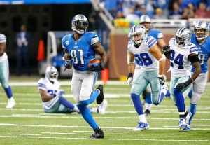
On Sunday, Calvin Johnson picked up 329 receiving yards against the Cowboys, the second most receiving yards in a single game after Flipper Anderson’s 336 yards in 1989 against the Saints. But when I think of the greatest games by a receiver of all time, my mind instantly goes to a performance by Kansas City’s Stephone Paige in a game in December 1985 against the Chargers. Regular readers will recall that this summer, Neil Paine and I developed a statistic known as True Receiving Yards. You can see a list of the leaders in TRY since 1950 here, but today I want to apply that same methodology on the single-game level. After crunching the numbers, Paige comes in at #2, Megatron’s performance comes in at #11, and Anderson is all the way down at #26. Why? How? Glad you asked. And I’ll keep the top spot a secret for now, in case anyone wants to guess.

1) First, we convert receiving yards into Adjusted Catch Yards by giving a five-yard bonus for receptions and a 20-yard bonus for touchdowns. Johnson had 419 ACY against the Cowboys, tied with Jerry Rice (against the ’95 Vikings) for the third highest mark since 1960.  The top spot belongs to Anderson at 431 (and personal favorite Jimmy Smith holds the number two spot for his performance against the 2000 Ravens). Paige — who produced an 8-309-2 stat line — totaled 389 Adjusted Catch Yards.

2) Next, we convert back to receiving yards by multiplying each receiver’s ACY by the league average ratio of receiving yards to Adjusted Catch Yards in that season. The point of using ACY instead of receiving yards is to include things other than receiving yards, but we still want to convert back into receiving yards. In 1985, the ACY/RecYd ratio was 0.66, in ’89 it was 0.66, and through eight weeks, that number is 0.65 in 2013, so not much is changing here. After step two, Anderson is at 286.6 receiving yards, Johnson 270.9 yards, and Paige 258.0 yards.

3) The third step is the pass attempts adjustment. The league average team team this year has averaged 38.7 attempts (including sacks) in 2013, while Matthew Stafford had 49 dropbacks yesterday. This means the Lions passed 26.6% more often than the average team. So what sort of adjustment do we make? In True Receiving Yards version 2.0, we split that number in half. I tried that here, and honestly, the numbers just didn’t look right — the top of the list was almost exclusively players on teams that had 10 or 12 pass attempts in that game. So instead of contracting the difference between pass attempts and league average pass attempts by two, I’m going to do it by three. So Johnson only gets downgraded to 91.1% of his production, or 246.9 yards.

Anderson’s record-breaking performance came in overtime in a game the Rams trailed by 14 entering the fourth quarter. As a result, Jim Everett had 57 dropbacks in a time period when 34.5 attempts was the norm.  So with Los Angeles having 65.3% more attempts than the average team that year, we have to lower Anderson from 286.6 to 224.1.

Paige, meanwhile, goes far in the other direction. The Chiefs took a 35-3 second quarter lead that day — in no small part due to Paige’s touchdown receptions of 56 and 84 yards — so Kansas City was limited to just 24 dropbacks. The average number of dropbacks in ’85 was 35.1, putting the Chiefs at just 68.4% of league average. Therefore, we bump up Paige by 15.4%, vaulting him from 258 yards to 297.9.

4) The final adjustment is the era adjustment. I’m going to use a different way to incorporate era adjustments here, because while passing yards have shot through the roof, the value of a team’s #1 wide receiver has been much less volatile. So I used the following baseline for each year: the number of Adjusted Catch Yards in the Nth best receiving game, when 2N = the number of team games in that season. So in modern times, with 512 games, this means the 256th highest ACY total in that season is the baseline; in 2011 and 2012, that was 135 Adjusted Catch Yards. From 1960 to 2012, the average was 124.3. ^[1]Note: I was lazy, and combined the AFL and NFL. I know, I know.

So what we do now is multiply each receiver’s score from step three by the baseline for that year, and divide by 124.3. I will use the same 135 as the baseline for 2013, which brings Megatron to 227. The baseline in ’89 was 130, so Anderson goes to 214.3, and in ’85, the baseline was 125, so Paige only drops to 296.2.

If you’ve made it this far, then maybe I’m not a complete idiot for putting the fine print up front. Without further ado, here are the top 250 ^[2]Note. I excluded two games during the 1987 strike played with replacement players: Anthony Allen had 262 TRY against the Cardinals, and Steve Largent had 260 TRY in Detroit. performances since 1960 using this formula:
[continue reading…]

Suppose you watch an entire football game. Your job is to put a single number on the degree to which the winning team beat the losing team. Qualitatively, the scale runs from “had any number of things gone differently at the end, the winning team would have lost” to “the winning team was in control for most of the game” to “this game was never in question.”

I want to quantify that qualitative scale. And I want to do it in a retrodictive way. In other words, I’m not as interested in the degree to which the winning team outplayed the losing team as I am in the degree to which the winning team was in control of the game. To see the difference, imagine a game where one team opens up a 14-0 lead on a kickoff return touchdown and a fluke turnover that leads to a score, then cruises to an uneventful 31-17 win. The advanced stats might even show that the losing team was more efficient. The predictive measures might give the losing team a better grade, because the reasons the winning team won were not things that are likely to carry over to future games. I don’t care about any of that. The kick return happened, and the turnover happened, and the result was that the game was never in any serious doubt.

The easiest way to do this is to use margin of victory, and that works well in most cases, but there are obvious outliers. Consider the Green Bay – Washington game from week two, which was 24-0 midway through the second quarter and never really got any closer, and the Colts-49ers game, which was a one-score game with five minutes remaining. The latter game finished with a larger margin of victory. Again, if you’re interested in predictive measures, you probably do want to record that Robert Griffin III was able to generate a couple of late TDs and that the Colts were able to put away the 49ers so quickly and thoroughly. But I’m not interested in that here.

Another natural answer would be to use Chase’s game scripts. Or, if you wanted to fancy up the same concept, you could compute the average win probability throughout the game. This too would work in the majority of cases, but not always. If a game is tied with two minutes left, that’s really all I need to know: the game should be graded as “could’ve gone either way.” But game scripts (or average WP) would be sensitive to how the game progressed for its first 58 minutes. Whether one team went up 21-0 and then the other team came back to tie it, or the game was a seesaw affair, all that really matters that the game was still very much in question at the end.

In 2008, I borrowed an idea that the great Matt Hinton called Time of Knockout. Chase later refined the idea with these two posts. Those were a couple more attempts to get at what I’m trying to get at above. These are fun, but they are flawed in ways similar to margin of victory and game script. The comments to Chase’s posts contain a lot of the ideas in the discussion above.

Now I’m going to tell you my answer. Then you’ll use the comments to tell me how to improve it. [continue reading…]

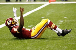
After a week six in which no team won with a negative Game Script, only the Jets won with a negative Game Script in week seven, and that was in overtime. Only two quarterbacks led fourth-quarter comebacks this week: Robert Griffin III and Thaddeus Lewis. Three more quarterbacks — Andy Dalton, Ben Roethlisberger, and Geno Smith — led game-winning drives in tie games, but in general, it was a pretty uneventful week for comebacks. Overall, it’s been a quit few weeks in the NFL when it comes to fourth quarter craziness: the largest deficit entering the 4th quarter by a winning team in weeks 5, 6, and 7 was just five points.

Just like last week, Alex Smith and the Chiefs pulled out a late win in a game with a near-even Game Script. None of the 13 other games this week (excluding Jets/Patriots, Chiefs/Texans, and noting that the Saints and Raiders had byes) had a Game Script of fewer than 2 points.
[continue reading…]

The Patriots and Pythagoras

With the exception of a blowout win over Tampa Bay, each Patriots game this year has been in doubt until the final minute. Against Buffalo, Stephen Gostkowski hit the game-winning 35-yard field goal with nine seconds left. In week two, the Jets had the ball, trailing by three, with 56 seconds remaining at their own 29-yard line, but a Geno Smith interception ended the comeback attempt. The Falcons failed on 4th-and-7 from the Patriots 10-yard line, trailing by a touchdown, with 41 seconds remaining. And last week, Tom Brady had not one, not two, but three chances to win the game in the final three minutes; eventually, he hit Kenbrell Thompkins with 10 seconds left for the game-winning touchdown.

To be fair, the Patriots sole loss was a nail-biter, too: it wasn’t until Adam Jones intercepted a Tom Brady pass at the Bengals three-yard line with 26 seconds remaining that Cincinnati sealed the 13-6 win. Still, New England has “only” outscored its opponents by 28 points so far this year. That’s a pretty low number for a 5-1 team.

From 1920 to 2012, 222 teams started the season with a 5-1-0 record. In an odd bit of trivia, the only one of those teams with a negative points differential through six games was a Super Bowl champion: the 1976 Oakland Raiders, who were blown out by the Patriots in week four but finished the year 16-1 (including a controversial revenge victory against New England in the playoffs).

If we limit ourselves to just post-merger teams, there are 148 teams that started 5-1-0 prior to 2013. If we throw out the strike seasons, that leaves us with 139 teams. This is the part of the post where you’d expect the teams with the highest points differential to perform the best over the rest of the season, but that actually hasn’t been the case.
[continue reading…]

I’ve posted the Game Scripts data following every week this season, but week six was the first week that no team won with a negative Game Script. That includes New England: even though Tom Brady led a late comeback, finding Kenbrell Thompkins in the back of the end zone to pull out a last-second win, the Patriots posted a Game Script score of +3.6. New England led 17-7 at halftime and for most of the second half; in fact, the Saints only held the lead for about seven minutes of game time. The third closest Game Script in week six comes courtesy of the Kansas City-Oakland matchup, which might surprise any of you who just saw the final 24-7 score. Of course, quirky games like that one is one of the reasons I came up with concept of Game Scripts.

The first score of the game was Terrelle Pryor’s 39-yard touchdown pass to Denarius Moore, with 8:47 left in the second quarter. This means for the first 21.2 minutes, the game was tied. Kansas City answered with a Jamaal Charles touchdown run with 1:12 left in the half, so the Raiders held a 7-point lead for 7.6 minutes. The Chiefs didn’t take their first lead of the game until Charles scored again with 2:07 left in the third, which means the game was tied for another 14.1 minutes. That score held for nearly 15 full minutes: Ryan Succop hit a short field goal with 2:13 left in the game. Pryor then threw a pick six with 1:45 left and the team down by 10, providing the final points in the 24-7 Kansas City victory.

All told, however, the game was tied for 35.3 minutes and the Raiders had a 7-point lead for 7.6 minutes, while the Chiefs led by 7 for 14.9 minutes, by 10 for 0.5 minutes, and by 17 for 1.7 minutes. That’s why the Game Script was just +1.4 for Kansas City, which is a much better reflection of how the game unfolded than the 24-7 final score. The table below shows the Game Scripts data for each contest in week six:
[continue reading…]

The New York Giants are now 0-6. There are many reasons for the team’s struggles: questionable drafting, injuries, Eli Manning interceptions, injuries, coaching mistakes by Tom Coughlin, and injuries. But let’s say you have a buddy who is convinced that the Giants are not that bad: in fact, he thinks New York is just a .500 team that has been really unlucky.

Your first inclination might be to stop being friends with this person, but after that, you might wonder: “Hey, how likely is it for a .500 team to start off 0-6?” This is the same (ignoring strength of schedule, the fact that games are not independent, and several other variables) as asking the question “how likely is a coin to land on heads six times in a row?” The answer to both questions is pretty simple: 0.500^6, or 1.56%. Using the binomial distribution (in Excel, this would involve typing =BINOM.DIST(0,6,0.5,TRUE) into a cell) — which assumes that the talent level of NFL teams is normally distributed, an assumption I will make throughout this post — would give you the same result of 1.56%.

That answer is simple, but it actually answers a different question. What you want to know is the likelihood that the Giants are actually a .500 or better team. It’s a minor but crucial distinction: what we just determined was the likelihood that, given the assumption that the Giants are a .500 team, that they would start 0-6. To address the question of how likely the 2013 Giants are actually a .500 (or better) team despite the 0-6 start, we need to use Bayes Theorem.

Much of the math involved in this process is frankly over my head, but fortunately, Kincaid over at 3-D baseball already did much of the work (and thanks to Neil for giving me that link). I will be blatantly copying his article (with the only changes being stylistic and making this for, you know, football), so make sure to give him all the credit he deserves. It’s a fantastic piece that has many useful applications.
[continue reading…]

I’ve been posting the Game Scripts numbers each week this season, and now have a full page dedicated to the results from every game at the top right of your screen. But the best use of Game Scripts is to adjust Pass ratios for teams to understand their true Passing Identity. Here’s how you do it.

1) Calculate how many standard deviations above/below average each team is in Game Scripts. The average Game Script, of course, is zero. The standard deviation through five weeks is 4.69, so the Broncos (8.43 Game Script) are 1.80 standard deviations above average in Game Script.

2) Calculate how many standard deviations from average each team is in Pass Ratio, defined as pass attempts (including sacks) divided by total plays. The average Pass Ratio through five weeks is 59.8%, while the standard deviation among the thirty-two teams is 6.7%. The Giants (excluding last night’s game) lead the league in Pass Ratio at 71.8%, which is 1.79 standard deviations above the league-average Pass Ratio.

3) Add how many standard deviations above/below average each team is in both Game Scripts and Pass Ratio. To convert these into an Index (and a more intuitive number for folks), multiply that result by 15 and add it to 100. So a team that has a Pass Identity that is 1 standard deviation above average will be at 115, while a team that is 1.6 standard deviations below average will be at 76.

Here are the results:
[continue reading…]

Last week, we announced that our True Receiving Yards metric has now been calculated back to 1950, so it’s only fitting that we also compute WOWY (With Or Without You) for all of those receivers as well.

Skip the paragraph after this if you don’t care about the gory mathematical details, and just know that WOWY basically answers the question: “Did a receiver’s quarterbacks play better when they threw a lot to him, or not?”

For the brave souls who care about the calculation: WOWY starts by measuring the difference between a QB’s age-adjusted Relative Adjusted Net Yards Per Attempt in a given season and his combined age-adjusted RANY/A in every other season of his career. This is computed as an average for each team’s QB corps, using a combination of QB dropbacks during the season in question and the rest of his career as the weights (the exact formula is: weight = 1/(1/drpbk_year + 1/drpbk_other)). Finally, for each receiver we compute a weighted career average of the QB WOWY scores for the teams he played on, weighted by his True Receiving Yards in each season.

At any rate, the only players who don’t get a WOWY are those who either debuted before 1950, played with a QB who debuted before 1950, or played with a QB who ever threw to a receiver who debuted before 1950. Here are the career WOWY marks (when applicable), alongside TRY, for every 3,000-TRY receiver whose career started in 1950 or later:

[continue reading…]

As Jason Lisk and I wrote about before the season, Tom Brady and Ben Roethlisberger have become something of the poster children so far this year when it comes to veteran QBs working with inexperienced and otherwise less-than-notable receiving groups. And, lo and behold, each has put up career-low RANY/A marks through 2 games. But how do their receiving corps rank relative to those of other teams so far this year, and how do they stack up historically?

To take a stab at answering these questions, I turned to True Receiving Yards. For each player who debuted in 1950 or later, I computed their Weighted Career True Receiving Yards for every year, as of the previous season, to get a sense of how experienced/accomplished they’d been going into the season in question. Then, I calculated a weighted averaged of those numbers for every receiver on a given team, using TRY during the season in question as the weights. For example, here are the 2013 Patriots receivers:

Player	Age	Debut	TRY	% of Tm	At-the-time WCTRY
Julian Edelman	27	2009	139	38%	615.7
Danny Amendola	28	2009	72	20%	1541.9
Kenbrell Thompkins	25	2013	56	15%	0.0
Shane Vereen	24	2011	44	12%	110.9
Aaron Dobson	22	2013	43	12%	0.0
Michael Hoomanawanui	25	2010	5	1%	278.8
James Develin	25	2013	4	1%	0.0
Weighted Average					560.7

The way to read that is: Julian Edelman has accounted for 38 percent of the Pats’ TRY so far. Going into the season, he had a career Weighted TRY of 615.7, so he contributes to 38% of the 2013 Pats’ weighted average with his 615.7 previous career weighted TRY; Danny Amendola contributes to 20% of the team weighted average with his 1541.9 previous career weighted TRY; etc. Multiply each guy’s previous weighted career TRYs by the percentage of the team’s 2013 TRY he contributed, and you get a cumulative weighted average of 560.7 — meaning the average TRY of a 2013 Pats receiver has been gained by a guy who had a previous career weighted TRY of 560.7.

Is that a low number? Well, here are the numbers for all of the 2013 team receiving corps (not including Thursday night’s Eagles-Chiefs tilt), inversely sorted by weighted average (asterisks indicate rookies):

[continue reading…]

About a month ago, Chase & I developed a stat called True Receiving Yards, which seeks to put all modern & historical receiving seasons on equal footing by adjusting for the league’s passing YPG environment & schedule length, plus the amount the player’s team passed (it’s easier to produce raw receiving stats on a team that throws a lot), with bonuses thrown in for touchdowns and receptions. It’s not perfect — what single stat in a sport with so many moving parts is? — but it does a pretty good job of measuring receiving productivity across different seasons and across teams with passing games that operated at vastly different volumes.

Anyway, today’s post is basically a data dump to let everyone know we’ve extended TRY data back to 1950 (before, it was only computed for post-merger seasons). Here are the new all-time career leaders among players who debuted in 1950 or later (see below for a key to the column abbreviations):
[continue reading…]

Tom Brady and the Patriots ran 89 plays in week one. Chip Kelly’s Eagles ran 53 plays in the first half. The Denver hurry-up offense picked up 510 yards, and would have run more than their 68 plays had Peyton Manning stopped throwing touchdowns and prematurely ending drives.

But if it seemed like week one was played at turbo speed, you probably didn’t watch the Seahawks-Panthers game. Carolina finished with a league-low 49 offensive plays. For those who didn’t closely monitor the coordinator situation in Carolina, here’s a bit of background. Rob Chudzinski was the Panthers offensive coordinator the past two seasons. His team’s inconsistent play and poor record drew ire from some fans, but the overall impressive nature of the Carolina offense landed him the top job in Cleveland. With head coach Ron Rivera on the hot seat, he simply promoted quarterbacks coach Mike Shula to offensive coordinator. Here’s what my buddy and Footballguys.com co-writer Jason Wood had to say about the change back in June:

Mike Shula last called plays in the NFL in 1999, his final season coaching under Tony Dungy in Tampa Bay. Since then, Shula is better known as the guy who preceded Nick Saban at the University of Alabama and less for his abilities as an NFL offensive difference maker. In spite of his limited recent experience, … it was his relationship with and tutelage of Cam Newton that made him the obvious choice for the OC position.

Schematically, Shula is keeping the foundation of Chudzinski’s offense in place, but in an effort to expedite the pace he has simplified the terminology. By doing so, Cam Newton can get in and out of the huddle far faster and the Panthers can try to dictate tempo in a way that was impossible a season ago. Cam Newton explained in a recent interview, “Twins Right, Key Left, 631 Smash M sounds completely different than Twins Right Tampa…It comes out of your mouth faster. You get in the huddle, it’s the same exact play.”

The early returns on the up-tempo offense are not good — how did the team run just 49 plays against Seattle? Carolina was one of the few teams to have success on the ground in week one — the Panthers rushed for 134 yards on 5.2 yards per carry, placing them in the top six in both metrics. And while Cam Newton didn’t have a great game, he completed 70% of his passes, which usually leads to lots of plays. How does a team that runs well and throws only seven incomplete passes score just 7 points and get limited to 49 plays? As it turns out, Mike Shula bears some of the blame.
[continue reading…]

In May, I wrote that the scoring team is responsible for roughly 60% of the points it scores, while the opponent is responsible for 40% of those points. In other words, offense and defense both matter, but offense tends to matter more.

I was wondering the same thing about passing yards. When Team A plays Team B, how many passing yards should we expect? As we all know, Team A can look very different when it has Dan Orlovsky instead of Peyton Manning, so I instead chose to look at Quarterback A against Team B. Here’s the fine print:

1) I limited my study to all quarterbacks since 1978 who started at least 14 games for one team. Then, I looked at the number of passing yards averaged by each quarterback during that season, excluding the final game of every year. I also calculated, for his opponent, that team’s average passing yards allowed per game in their first 15 games of the season.

2) I then calculated the number of passing yards averaged by each quarterback in his games that season excluding the game in question. This number, which is different for each quarterback in each game, is the “Expected Passing Yards” for each quarterback in each game. I also calculated the “Expected Passing Yards Allowed” by his opponent in each game, based upon the opponent’s average yards allowed total in their other 14 games.

3) I then subtracted the league average from the Expected Passing Yards and Expected Passing Yards Allowed, to come up with era-adjusted numbers.

4) I performed a regression analysis using Era-Adjusted Expected Passing Yards and Era-Adjusted Expected Passing Yards Allowed as my inputs. My output was the actual number of passing yards produced in that game.
[continue reading…]

In 1998, 21-year-old Randy Moss made a stunning NFL debut, racking up 17 touchdowns and 1,260 True Receiving Yards, the 2nd-best total in football that season. The Vikings’ primary quarterback that year, Randall Cunningham, was a former Pro Bowler and MVP, but all that seemed like a lifetime ago before the ’98 season. He’d been out of football entirely in 1996, and in 1997 he posted an Adjusted Net Yards per Attempt average that was 1.2 points below the league’s average (for reference’s sake, replacement level is usually around 0.75 below average). With Moss in ’98, though, Cunningham’s passing efficiency numbers exploded: he posted a career best +3.2 Relative Adjusted Net Yards per Attempt, miles ahead of his perfectly-average overall career mark. If we adjust for the fact that Cunningham was also 35 at the time (an age at which quarterbacks’ RANY/A rates tend to be 1.1 points below what they are at age 27), Cunningham’s 1998 rate was actually 4.3 points better than we’d expect from the rest of his career, a staggering outlier.

The following year, Jeff George took over as the Vikings primary quarterback, and he promptly posted a Relative ANY/A 2.2 points higher than expected based on his age and the rest of his career. ^[1]Cunningham’s RANY/A was also 1.0 better than expected in limited action. George left Moss and Minnesota after the season, and he would throw only 236 passes the rest of his career, producing a cumulative -0.6 RANY/A in Washington before retiring.

From 2000-04, Moss was the primary target of Daunte Culpepper, whose RANY/A was 0.7 better than expected (based on Culpepper’s career numbers) when Moss was around. ^[2]That number is an average weighted by the number of TRY Moss had in each season Although he’d enjoyed one of the best quarterback seasons in NFL history in 2004, Culpepper was never the same after Moss was traded to Oakland; in fact, he never even had another league-average passing season, producing a horrible -1.2 RANY/A from 2005 until his retirement in 2009. ^[3]To be fair, Culpepper tore his ACL, MCL, and PCL halfway through the 2005 season, which also was a factor in his decline.

Moss’s stint with the Raiders was famously checkered — although Kerry Collins’ RANY/A was 0.6 better than expected in 2005, Aaron Brooks played 2.5 points of RANY/A below his previous standards in 2006 — but we all know what happened when he joined the Patriots in 2007. With Moss, Tom Brady’s RANY/A was a whopping 1.3 points higher than expected from the rest of his career, and Moss also played a big role in Matt Cassel’s RANY/A being +1.0 relative to expectations after Brady was lost for the season in 2008.

While Moss’s post-Pats career hasn’t exactly been the stuff of legends, the majority of his career (weighted by True Receiving Yards) saw him dramatically improve his quarterbacks’ play relative to the rest of their careers. In fact, his lifetime WOWY (With or Without You) mark of +1.1 age-adjusted RANY/A ranks 3rd among all receivers who: a) had at least 3,000 career TRY, b) started their careers after the merger, and c) played exclusively with quarterbacks who started their careers after the merger. And the first two names on the list are possibly explained by other means. The table below lists all 301 receivers with 3,000 career TRY. The table is fully sortable and searchable, and you can click on the arrows at the bottom of the table to scroll. The table is sorted by the QB WOWY column.
[continue reading…]

While the state of the Steelers’ receiving corps isn’t as shaky as say, that of the New England Patriots, it could certainly be called an area of potential concern for Ben Roethlisberger and the Pittsburgh offense going into 2013. One of the biggest moves on the first day of free agency involved Mike Wallace departing for Miami; meanwhile, Heath Miller’s injury status — while more encouraging than previously thought — will cost him several games, and probably some effectiveness when he does eventually return. All of this comes on the heels of losing stealth HoFer Hines Ward (albeit an older, drastically less effective version) to retirement after the 2011 season.

For Roethlisberger, this downturn in the quality of his receivers is a pretty new phenomenon. In fact, by one measure of career receiving-corps talent (which I’ll explain below), Big Ben has been blessed with the fourth-most gifted receiving group among current starting quarterbacks with more than two years of experience (behind only Peyton Manning, Matt Ryan, and Tony Romo). In fact, Roethlisberger’s 16th-ranked receiving corps in 2012 was by far the least talented group of pass catchers he’s ever had to throw to.

How do you begin to measure the quality of a quarterback’s receiving corps, you ask? Well, pretty much any method is going to fraught with circular logic, especially if a quarterback consistently has the same receivers over several years. His successes are theirs, and vice-versa. However, here’s one stab at shedding at least some light on the issue.

For each team since the NFL-AFL merger, I:

• Gathered all players with at least 1 catch for the team in the season.
• Computed their True Receiving Yards in that season; I then determined what percentage of the team’s True Receiving Yards was accumulated by which receiver in each year. For example, Hines Ward had 1,029 TRY in 2009, which represented 25.9% of the 3,979 True Receiving Yards accumulated by all Steelers that year
• Figured out the most TRY they ever had in a season, a number I’m calling each player’s peak TRY; for Ward, his peak TRY is equal to 1,279.
• Calculated a weighted average (based on the percentage of team TRY gained by each receiver) of the receivers’ peak TRY (weighted by their TRY during the season in question).

(I also threw out all teams that had a receiver who debuted before 1970, since I don’t know what the real peak TRY of any pre-merger receiver was. I should eventually calculate TRY for pre-merger seasons, of course — thank you Chase & Don Maynard.)

As an example, here are the 2009 Steelers, the most talented corps of receivers Roethlisberger has had in his career:
[continue reading…]

As you guys know, Neil Paine is the man. Here’s the latest reason: he came up with a metric called True Receiving Yards, the latest in a long line of thoughts in our Wide Receiver Project. So, what are True Receiving Yards?

We start with Adjusted Catch Yards, defined as 5 * Receptions + Receiving Yards + 20 * Receiving Touchdowns.

1) Then, we convert each player’s Adjusted Catch Yards to the same scale as pure receiving yards using the following formula:

Adjusted Catch Yards * League Receiving Yards / League Adjusted Catch Yards

2) Next, we adjust for how often the receiver’s team passed.  We use the following formula:

[Result in Step 1] * League_Avg_Team_Pass_Attempts / Team_Pass_Attempts

For purposes of this post, Team Pass Attempts include sacks.

3) Then we adjust for the league passing environment, by using this formula:

[Result in Step 2] * by (214.54/Avg_Team_Receiving_Yards_Per_Game).

Why 214.54? Because that’s how many yards the average NFL team has passed for in each season since 1970.

4) Finally, we need to adjust for schedule length. This one’s pretty simple:

[Result in Step 2] * 16 / Team Games

As it turns out, the single-season leader in True Receiving Yards is….. Harold Jackson for the 1973 Rams. That will probably surprise some folks; heck, it surprised me. So let’s walk through Jackson’s season by comparing it to Calvin Johnson’s 2012. Jackson caught 40 passes for 874 yards and 13 touchdowns. That gives him 1,334 Adjusted Catch Yards, while Megatron’s 122-1964-5 translates to 2,674 Adjusted Catch Yards, more than twice what Jackson produced.

1) First, we need to convert those ACY numbers into receiving yards.  In 1973, that conversion ratio is 65.5%, and in 2012, it was 64.5%; this means Jackson is credited with 874 receiving yards (ironically, his actual number) while Johnson is pushed down to only 1,725 yards. This is because Johnson had a ton of yards but only five touchdowns.  In other words, based on his receptions, receiving yards, and receiving touchdowns, Johnson was more like a 1,725-yard receiver last year.

2) Jackson’s Rams had just 288 Team Pass Attempts, while the average team in 1973 averaged 373.3 pass attempts. So we need to bump Jackson up by 29.6%, which would give him 1,132 receiving yards. The 2012 Lions had 769 Team Pass Attempts compared to a league average of 592.4; therefore, we need to give Johnson credit for only 77% of his ACY, bringing him down to 1,329 receiving yards.

3) Next, we adjust for league environment. In 1973, the average team passed for 159 yards per game, which means we need to bump Jackson up by 34.6% (the result of 214.54 divided by 159); this gives him 1,524 receiving yards. For Megatron, since the average team in 2012 passed for 246 yards per game, we need to multiply his result in step 2 by 87.2%, leaving him with only 1,159 receiving yards.

4) For Calvin Johnson, that’s it: he is credited with 1,159 True Receiving Yards, after reducing his numbers for playing in a pass-happy offense, playing in a pass-happy era, and not having many touchdowns. For Jackson, his 1,524 gets pro-rated to a 16-game season, giving him 1,742 True Receiving Yards.
[continue reading…]

Yesterday, I set up a method for ranking the flukiest fantasy football seasons since the NFL-AFL merger, finding players who had elite fantasy seasons that were completely out of step with the rest of their careers. I highlighted fluke years #21-30, so here’s a recap of the rankings thus far:

30. Lorenzo White, 1992
29. Dwight Clark, 1982
28. Willie Parker, 2006
27. Lynn Dickey, 1983
26. Robert Brooks, 1995
25. Ricky Williams, 2002
24. Jamal Lewis, 2003
23. Mark Brunell, 1996
22. Vinny Testaverde, 1996
21. Garrison Hearst, 1998

Now, let’s get to…

The Top Twenty

20. RB Natrone Means, 1994

Best Season
year	g	rush	rushyd	rushtd	rec	recyd	rectd	VBD
1994	16	343	1,350	12	39	235	0	103.0
2nd-Best Season
year	g	rush	rushyd	rushtd	rec	recyd	rectd	VBD
1997	14	244	823	9	15	104	0	12.9

Big, bruising Natrone Means burst onto the scene in 1994 as a newly-minted starter for the Chargers’ eventual Super Bowl team, gaining 1,350 yards on the ground with 12 TDs. In the pantheon of massive backs, he was supposed to be the AFC’s answer to the Rams’ Jerome Bettis, but Means was slowed by a groin injury the following year and never really stayed healthy enough to recapture his old form. The best he could do was to post a pair of 800-yard rushing campaigns for the Jaguars & Chargers in 1997 & ’98 before retiring after the ’99 season.

19. WR Braylon Edwards, 2007

Best Season
year	g	rec	recyd	rectd	VBD
2007	16	80	1,289	16	107.7
2nd-Best Season
year	g	rec	recyd	rectd	VBD
2010	16	53	904	7	15.4

The 3rd overall pick in the 2005 Draft out of Michigan, Edwards seemingly had a breakout 2007 season catching passes from fellow Pro Bowler Derek Anderson. But both dropped off significantly the next season, and Edwards was sent packing to the Jets in 2009. He did post 904 yards as a legit starting fantasy wideout in 2010, but he has just 380 receiving yards over the past 2 seasons, and it’s not clear he’ll ever live up to those eye-popping 2007 numbers again.
[continue reading…]

There’s nothing like a truly great fluke fantasy season. Because they can help carry you to a league championship (and therefore eternal bragging rights — flags fly forever, after all), a random player who unexpectedly has a great season will often have a special place in the heart of every winning owner. And even if you only use their jerseys as makeshift aprons to cook in, fluke fantasy greats are a part of the fabric of football fandom. That’s why this post is a tribute to the greatest, most bizarre, fluke fantasy seasons of all time (or at least since the 1970 NFL-AFL merger).

First, a bit about the methodology. I’m going to use a very basic fantasy scoring system for the purposes of this post:

• 1 point for every 20 passing yards
• 1 point for every 10 rushing or receiving yards
• 6 points for every rushing or receiving TD
• 4 points for every passing TD
• -2 points for every passing INT

I’m also measuring players based on Value Based Drafting (VBD) points rather than raw points. In a nutshell, VBD measures true fantasy value by comparing a player to replacement level, defined here as the number of fantasy points scored by the least valuable starter in your league. For the purposes of this exercise, I’m basing VBD on a 12-team league with a starting lineup of one QB, two RBs, 2.5 WRs, and 1 TE. That means we’re comparing a player at a given position to the #12-ranked QB, the #24 RB, the #30 WR, or the #12 TE in each season. If a player’s VBD is below the replacement threshold at his position, he simply gets a VBD of zero for the year.
[continue reading…]

Back in March, Chase wrote a post investigating how quarterbacks age, finding that they peak at age 29 (with a generalized peak from 26-30) in terms of value over average. Today, I thought I’d quickly look at how quarterbacks age in terms of their performance rate — specifically, their Adjusted Net Yards per Attempt (ANY/A). For newer readers, ANY/A is based on the following formula: (Passing Yards + 20 * Passing TDs – 45 * INTs – Sack Yards Lost) / (Pass Attempts + Sacks).

First, I need to introduce a way of adjusting ANY/A for era: Relative ANY/A. Relative ANY/A is simply equal to:

QB_ANY/A – LgAvg_ANY/A

The table below lists the 30 single-season leaders in Relative ANY/A since the merger. You won’t be too surprised to see the 2004 version of Peyton Manning at the top. That year, Manning averaged 9.8 ANY/A, while the league average was just 5.6 ANY/A. That means Manning gets a Relative ANY/A grade of +4.1 (with the difference due to rounding).
[continue reading…]

Here is a recap of the 2012 Chicago Bears season.  Notice anything strange? Trick question!

[continue reading…]

Yesterday, I presented my Rearview ANY/A ratings for quarterbacks and defenses in 2012. Strength of schedule adjustments are important — without it, Peyton Manning‘s numbers were tops in the league, but after the adjustments, Tom Brady moved into the number one slot. To create the season rankings, I had to come up with rankings for each quarterback and each defense in every game last season, so I figured I should present those results as well.

Using the same principles from yesterday’s post, the table below shows all games where a quarterback produced over 100 Adjusted Net Yards above average. You’re probably surprised to see that Chad Henne’s performance in Houston ranks as the single best passing game of 2012. There were only 64 pass plays of 60+ yards last season, but three of them came by Henne against the Texans. That game narrowly edged out Brady’s Thanksgiving Night performance against the Jets (overshadowed by Le Buttfumble), and a separate shredding of the Texans secondary, this time courtesy of Aaron Rodgers. You can click on the boxscore below to see the full PFR boxscore of each game. As always, the table is fully searchable and sortable, and you can click the arrows at the bottom to see more rows.
[continue reading…]