≡ Menu

Every year at Footballguys.com, I publish an article called Rearview QB, which adjusts quarterback (and defense) fantasy numbers for strength of schedule. I’ve also done the same thing using ANY/A instead of fantasy points, and today I revive that concept for the 2012 season.

Let’s start with the basics. Adjusted Net Yards per Attempt is defined as (Passing Yards + 20 * Passing Touchdowns – 45 * Interceptions – Sack Yards Lost) divided by (Pass Attempts plus Sacks). ANY/A is my favorite explanatory passing statistic — it is very good at telling you the amount of value provided (or not provided) by a passer in a given game, season, or career.

Let’s start with some basic information. The league average ANY/A in 2012 was 5.93. Peyton Manning averaged 7.89 ANY/A last year, the highest rate in the league among the 39 passers with at least 75 attempts. Since the Broncos star had 583 pass attempts and 21 sacks in 2012, that means he was producing 1.96 ANY/A over league average on 604 dropbacks. That means Manning is credited with 1,185 Adjusted Net Yards above average, a metric I simply call “VALUE” in the table below. Manning led the league in that category, with Tom Brady, Drew Brees, Aaron Rodgers, and Matt Ryan rounding out the top five. Remember, the ANY/A and VALUE results aren’t supposed to surprise you, so it makes sense that the best quarterbacks finish near the top in this category every year.
[continue reading…]

{ 21 comments }

Last week, I wrote about why I was not concerned with Trent Richardson’s yards per carry average last season. I like using rushing yards because rush attempts themselves are indicators of quality, although it’s not like I think yards per carry is useless — just overrated. One problem with YPC is that it’s not very stable from year to year. In an article on regression to the mean, I highlighted how yards per carry was particularly vulnerable to this concept. Here’s that chart again — the blue line represents yards per carry in Year N, and the red line shows YPC in Year N+1. As you can see, there’s a significant pull towards the mean for all YPC averages.

regression ypc

I decided to take another stab at examining YPC averages today.  I looked at all running backs since 1970 who recorded at least 50 carries for the same team in consecutive years. Using yards per carry in Year N as my input, I ran a regression to determine the best-fit estimate of yards per carry in Year N+1. The R^2 was just 0.11, and the best fit equation was:

2.61 + 0.34 * Year_N_YPC

So a player who averages 4.00 yards per carry in Year N should be expected to average 3.96 YPC in Year N+1, while a 5.00 YPC runner is only projected at 4.30 the following year.

What if we increase the minimums to 100 carries in both years? Nothing really changes: the R^2 remains at 0.11, and the best-fit formula becomes:

2.63 + 0.34 * Year_N_YPC

150 carries? The R^2 is 0.13, and the best-fit formula becomes:

2.54 + 0.37 * Year_N_YPC

200 carries? The R^2 stays at 0.13, and the best-fit formula becomes:

2.61 + 0.36 * Year_N_YPC

Even at a minimum of 250 carries in both years, little changes. The R^2 is still stuck on 0.13, and the best-fit formula is:

2.68 + 0.37 * Year_N_YPC

O.J. Simpson typifies some of the issues. It’s easy to think of him as a great running back, but starting in 1972, his YPC went from 4.3 to 6.0 to 4.2 to 5.5 to 5.2 to 4.4. Barry Sanders had a similar stretch from ’93 to ’98, bouncing around from 4.6 to 5.7 to 4.8 to 5.1 to 6.1 and then finally 4.3. Kevan Barlow averaged 5.1 YPC in 2003 and then 3.4 YPC in 2004, while Christian Okoye jumped from 3.3 to 4.6 from 1990 to 1991.
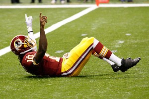
This guy knows about leading the league

This guy knows about leading the league.

Those are isolated examples, but that’s the point of running the regression. In general, yards per carry is not a very sticky metric. At least, it’s not nearly as sticky as you might think.

That was going to be the full post, but then I wondered how sticky other metrics are.  What about our favorite basic measure of passing efficiency, Net Yards per Attempt? For purposes of this post, an Attempt is defined as either a pass attempt or a sack.

I looked at all quarterbacks since 1970 who recorded at least 100 Attempts for the same team in consecutive years. Using NY/A in Year N as my input, I ran a regression to determine the best-fit estimate of NY/A in Year N+1. The R^2 was 0.24, and the best fit equation was:

3.03 + 0.49 * Year_N_NY/A

This means that a quarterback who averages 6.00 Net Yards per Attempt in Year N should be expected to average 5.97 YPC in Year N+1, while a 7.00 NY/A QB is projected at 6.45 in Year N+1.

What if we increase the minimums to 200 attempts in both years? It has a minor effect, bringing the R^2 up to 0.27, and producing the following equation:

2.94 + 0.51 * Year_N_NY/A

300 Attempts? The R^2 becomes 0.28, and the best-fit formula is now:

2.94 + 0.53 * Year_N_NY/A

400 Attempts? An R^2 of 0.26 and a best-fit formula of:

3.18 + 0.50 * Year_N_NY/A

After that, the sample size becomes too small, but the takeaway is pretty clear: for every additional yard a quarterback produces in Year N, he should be expected to produce another half-yard in NY/A the following year.

So does this mean NY/A is sticky and YPC is not? I’m not so sure what to make of the results here. I have some more thoughts, but first, please leave your ideas and takeaways in the comments.

{ 9 comments }

Wilson scrambles and gets credit for it.

Wilson scrambles and gets credit for it.

I hate passer rating. So do you. Everyone does, except for Kerry Byrne. Passer rating is stupid because it gives a 20-yard bonus for each completion, a 100-yard penalty for each interception, and an 80-yard bonus for each touchdown. In reality, there should be no (or a very small) weight on completions, a 45-yard weight on interceptions, and a 20-yard weight on touchdowns.

But let’s ignore those issues today. Reading Mike Tanier’s recent article inspired me to make see what passer rating would look like if we make three tweaks. I’m not going to change any of the weights in the formula, but just redefine the variables.

1) There’s no reason to exclude sack data from passer rating. I’ve stopped writing about how sacks are just as much (if not more) on the quarterback than other passing metrics, because I think that horse has been pretty well beaten by Jason Lisk and me.

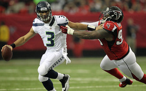
2) Scrambles should be treated like completed passes. If Russell Wilson is about to be sacked, but escapes and run for 7 yards, why should that be treated any differently than if Peyton Manning is about to be sacked, but throws a seven-yard pass at the last second?

3) Lost Fumbles should be counted with interceptions. One could make a few advanced arguments here — we should use all fumbles instead of lost fumbles, or fumbles should be given an even stronger weight than interceptions (although consider that in light of this post), or that we should limit ourselves to just fumbles lost on passing plays. I’m going to play the simple card here, and just use lost fumbles data on the season level.

Passer rating consists of four metrics, all weighted equally: completions per attempt, yards per attempt, touchdowns per attempt, and interceptions per attempt. I will use the same formula with the same weights and the same variables, but redefine what those variables are. Here are the new definitions, with the additions in blue.

Completion percentage is now (Completions plus Scrambles) / (Pass Attempts plus Sacks plus Scrambles)

Yards per Attempt is now (Passing Yards plus Yards on Scrambles minus Sack Yards Lost) / (Pass Attempts plus Sacks plus Scrambles)

Touchdown Rate is now (Passing Touchdowns plus Touchdowns on Scrambles) / (Pass Attempts plus Sacks plus Scrambles)

Turnover Rate will replace Interception Rate in the formula, and is calculated as (Interceptions plus Fumbles Lost) / (Pass Attempts plus Sacks plus Scrambles)

The table below lists all of those metrics for the 32 quarterbacks who had enough pass attempts to qualify for the passer rating crown, along with Alex Smith and Colin Kaepernick, who just missed qualifying. Let’s look at the Robert Griffin III line.

He completed 258 of 393 pass attempts for 3200 yards, with 20 touchdowns and five interceptions. Those are the standard stats that make up passer rating, but he also took 30 sacks and lost 217 yards on those sacks. That makes Griffin’s numbers worse, but he also had 38 scrambles for 302 yards (which gets recorded as 38 completed passes for 302 yards), with no scramble touchdowns. Finally, he lost two fumbles. His new completion percentage is 64.2%, his new yards per attempt is 7.13, his new touchdown rate is 4.3%, and his turnover rate (which includes fumbles) is 1.5%. The final two columns show each quarterback’s passer rating under the normal system and their passer rating using these metrics, which I’ll call the FPPR for short.
[continue reading…]

{ 14 comments }

Fantasy Football: Expected VBD (FBG)

[Note: For the rest of the year, content over at Footballguys.com is subscriber-only.]

Over at Footballguys.com, I build upon Joe Bryant’s VBD and create the idea of Expected VBD. While VBD is a great way to understand the value of players, Expected VBD explains how we draft. This concept is why even though you may expect some kickers and fantasy defenses to perform well, you don’t take them early in the draft because they have low Expected VBDs. So what is Expected VBD?

Instead of drafting according to strict VBD, you should be drafting to something I’ll call Expected VBD, which is best defined by an example. Suppose Russell Wilson has three equally possible outcomes this year: he has a one-in-three chance of scoring 425 fantasy points, 325 fantasy points, and 225 fantasy points. Further, let’s assume that the baseline number of fantasy points at the quarterback position is 300 fantasy points.

We would project Wilson to score 325 points, which would be the weighted average of his possible outcomes. This means VBD would tell you that he is worth 25 points, because 325 is 25 points above the baseline. Expected VBD works like this: If Wilson scores 425 points, he’ll produce 125 points of VBD. If he scores only 325 points, he’ll be worth +25, and if he scores only 225 points, he’s going to have -125 points of VBD. In real life, players with negative VBD scores can be released or put on your bench. So if Wilson scores 225 points (probably due to injury), you’ll start another quarterback, roughly a quarterback who can give you baseline production.

So when Wilson scores 225 fantasy points, his VBD is 0, not -75. That means his Expected VBD would be (125+25+0)/3, or 50. Wilson’s VBD according to our projections may be only 25, but his Expected VBD is twice as large because Expected VBD does not provide an extra penalty for sub-baseline performances. Not surprisingly, different positions have different amounts of Expected VBD associated with them.

Below is the summary graph — it has quickly become one of my all-time favorite graphs — which shows the Expected VBD by each position according to Average Draft Position.

ExpectedVBDADP

I go into much more detail in the full article.

{ 10 comments }

Knockouts in the NFL

I'm gonna Gronk you out

I'm gonna Gronk you out.

Three years ago, I posted a list of Approximate Times of Knockout in the NFL: I defined the time of a knockout as how much time was remaining in every game when the winning team first scored more points than the losing team ultimately scored by the end of the game.

I want to revisit the issue but use a slightly different formula. Since we have robust play-by-play data going back to 2000, I thought we could get more precise. In this post, I am defining the time of knockout as the last time the eventual losing team had the ball within one score of the eventual winning team. This seems to fit the definition of knockout a little bit better, I think, although it’s certainly not perfect. I went through every game of the 2012 season and recorded the time of knockout for the victor in each game. If you lost a game and last had the ball trailing within one score with 5 minutes left in the 3rd quarter, that goes down as a knockout with 20 minutes remaining. For the winning team, they get +20, while the loser gets -20. If you do that for every game, you can get season ratings.

Let’s take a look at the Patriots. They went 12-4 last year, and had an average net time of knockout of 19.4 minutes. The “net” means this includes losses in there as well. In their 12 wins, the Pats had an average time of knockout of 26.3 minutes, while in their four losses, they were knocked out with just over one minute remaining, on average. The Patriots had the highest average net time of knockout, but you might be surprised to see who had the highest average time of knockout in victories:
[continue reading…]

{ 5 comments }

Smith has excelled despite playing for a ground-based attack

Smith has excelled despite playing for a ground-based attack.

We don’t rank quarterbacks by passing yards because “passing yards” is largely a function of pass attempts. The same is true for receiving yards, as the number of times a team passes the ball has a big impact on a receiver’s yardage total. I’ve spent some time this year looking at ways to rank wide receivers and am throwing another log on that fire today. One idea I like in theory is receiving yards per team pass attempt, as it helps to solve the problem of dealing with receivers who play on pass-heavy teams.

But there are some obvious drawbacks to that approach. There are more passing options on the field now than ever before, so it’s tough to use receiving yards per team pass attempt across eras. For example, Jim Benton in 1945 owns the record in this metric at 5.36 yards per team attempt in 1945; even if you consider that high number a byproduct of World War II, Harlon Hill averaged 4.5 yards per team pass in 1956 for the Bears. Carolina’s Steve Smith is the single-season leader in yards per team attempt since 1970. And he also holds down the #2 on that list. Smith averaged 3.48 yards per team pass attempt in 2005; three years later, he averaged 3.43 Yd/TPA (but in the 14 games he played, Smith averaged an absurd 4.04 Yd/TPA).

A few weeks ago, I ranked receivers by their percentage of team receiving yards in their best six seasons. I thought it would be fun to do the same thing with yards per team pass attempt (excluding sacks). The results are listed below for the top 200 receivers; I’ve also included the six years selected for each receiver to come up with their average. As always, you can use the search box to find your favorite receiver, and the table is sortable, too. [1]Note that I am only giving a receiver credit for his receiving yards with each team in each season, so for say, Wes Chandler, his 1981 season is undervalued.
[continue reading…]

References

References
1 Note that I am only giving a receiver credit for his receiving yards with each team in each season, so for say, Wes Chandler, his 1981 season is undervalued.
{ 18 comments }

Yards per Attempt is the basic statistic around which the passing game should be measured. It forms the base of my favorite predictive statistic (Net Yards per Attempt) and my favorite explanatory statistic (Adjusted Net Yards per Attempt). But it’s not perfect.

In theory, Yards per Attempt is a system-neutral metric. If you play in a conservative, horizontal offense, you can have a very high completion percentage, like David Carr in 2006. But if you’re not any good (like Carr in 2006), you’ll produce a low yards-per-completion average, dragging down your Y/A average. You can’t really “game” the system to get a high yards per attempt average; the way to finish among the league leaders in Y/A is simply by being very good.

Courtesy of NFLGSIS, I have information on the length of each pass (or Air Yards) thrown during the 2012 regular season. I then calculated, for each distance in the air, the average completion percentage and average yards per completion. In the graph below, the X-Axis shows how far form the line of scrimmage the pass went (or, as Mike Clay calls it, the depth of target). The blue line shows the average completion percentage (off the left Y-Axis) based on the distance of the throw, while the red line shows the average yards per completion (off the right Y-Axis). For example, passes four yards past the LOS are completed 69% of the time and gain 5.4 yards per completion, while 14-yard passes are at 50% and 17.6.

Cmp vs. YPC2

We can also follow up on yesterday’s post by looking at Air Yards vs. YAC for each distance or depth of throw. Air Yards is in red and on the right Y-Axis, while average yards after the catch is in blue and measured against the left Y-Axis. Initially, there is a pretty strong inverse relationship, just like with completion percentage and yards per completion. On a completion that is one yard past the line of scrimmage, the average YAC is 5.5; on a completion 10 yards downfield, the average YAC drops to 3.0. This is why players like Percy Harvin and Randall Cobb will rack up huge YAC numbers. But once you get past 13 or 14 yards, YAC starts to rise again. This makes sense, as that far down the field, a player is just one broken tackle away from a huge gain (I suspect using median YAC might paint a different picture).
[continue reading…]

{ 16 comments }

Over at Footballguys.com, I look at a different method to project receiving yards.

The number of receiving yards a player produces is the result of a large number of variables. Some of them, like the receiver’s ability, are pretty consistent from year to year. But other factors are less reliable, or less “sticky” from year to year. I thought it would be informative to look at three key variables that impact the number of yards a wide receiver gains and measure how “sticky” they are from year to year. These three variables are:

  • The number of pass attempts by his team;
  • The percentage of his team’s passes that go to him; and
  • The receiver’s average gain on passes that go to him.

We can redefine receiving yards to equal the following equation:

Receiving yards = Receiving Yards/Target x Targets/Team_Pass_Att x Team_Pass_Att.

You’ll notice that Targets and Team Pass Attempts are in both the numerator and denominator of one of the fractions, and they will cancel each other out: that’s why this formula is equivalent to receiving yards.

By breaking out receiving yards into these three variables, we can then examine the stickiness of each one, which should help our Year N+1 projections. Below are the best-fit equations for each of those variables in Year N+1:

Future Pass Attempts = 36 + (450 x Pass_Attempts/Play) + (0.255 x Offensive Plays)

Future Percentage of Targets = 6.2% + 71.3% x Past Percentage of Targets

Future Yards/Target = 5.5 + 0.29 x Past Yards/Targets

I then used those three equations to come up with a starting point for receiving yards projections for 28 wide receivers. You can read the full article here.

{ 0 comments }

The Dungy Index: Version 2.0

Each coach is given bonus points for mustaches.

Each coach is given bonus points for mustaches.

Back in 2006, Doug Drinen came up with the Dungy Index, a way to measure a coach’s performance in the regular season relative to expectations. Because Doug understands regression to the mean, he was impressed by Tony Dungy’s ability to continue to string together 12-win seasons year after year. [1]Admittedly, this looks less impressive when you consider that Jim Mora, Jim Caldwell, and John Fox have won 13+ games with Peyton Manning, too. But Doug didn’t want to just use winning percentage to rate coaches: expectations are lower when a coach inherits a bad team, and that needs to be taken into account.

Defining “expectations” is challenging. I don’t have a perfect way, but I do have a simple one: use a linear regression based off of last year’s Pythagorean winning percentage to predict the number of games a team should be expected to win this year. [2]All ties are counted as half-wins. I did just that, and the best-fit formula was:

Year N+1 Wins = 4.23 + 0.472 * Year N Wins

So a 3-win team should be expected to win 5.6 games in Year N+1, a 10-win team is projected at 9.0 wins, and a 13-win team drops down to 10.4 expected wins. If you subtract the number of expected wins from the number of actual wins by the coach in a season, you are left with his number of wins over expectation. You’ll see pretty quickly why this is called the Dungy Index: he fares very, very well in it.
[continue reading…]

References

References
1 Admittedly, this looks less impressive when you consider that Jim Mora, Jim Caldwell, and John Fox have won 13+ games with Peyton Manning, too.
2 All ties are counted as half-wins.
{ 15 comments }

Vegas likes Alabama a lot more than it likes LSU

Vegas likes Alabama a lot more than it likes LSU.

The Simple Rating System is a set of computer rankings focused on only two variables: strength of schedule and margin of victory. I published weekly college football SRS ratings each week last season, and you can read more about the SRS there. Last month, Jason Lisk of the Big Lead took the Las Vegas point spread for each NFL game to come up with a set of power rankings; I stole Lisk’s idea and used the same point spreads to create implied SRS ratings for every NFL team. The idea is that if the 49ers are a 10.5-point neutral site favorite over the Jaguars, that’s one data point that implies that Las Vegas views San Francisco as 10.5 points better than Jacksonville. By taking every data point, and using Excel to iterate the ratings hundreds of times, you can create a set of implied team ratings.

Last week, the Golden Nugget released the point spreads for 248 college football games. By using the same process, those point spreads can help us determine the implied ratings that Las Vegas has assigned to each team.

We don’t have a full slate of games, but we do have at least 1 game for 83 different teams. Theoretically, this is different than using actual game results: one game can be enough to come up with Vegas’ implied rating for the team. That’s because once we’re confident in Oklahoma’s rating, Tulsa being 18-point underdogs in Norman gives us a good estimate for how Vegas views Tulsa. I assigned 3 points to the road team in each game in coming up with the implied SRS ratings. For example, Arizona is an 11-point favorite on the road against California. So for that game, we assume Vegas believes the Wildcats are 14 points better than the Golden Bears; if we do this for each of the other 247 games, and then iterate the results hundreds of times, we can come up with a set of power ratings.

Unsurprisingly, Alabama comes out as the highest-rated team. The Crimson Tide are being rated as 19.6 points better than “average,” although average isn’t really a concept with much meaning here. The SRS rating has little meaning in the abstract, but is useful to get a sense of the Crimson Tide’s rating relative to the rest of the teams. If Alabama is 10 points better in the SRS than a team, that means Alabama would be projected as a 10-point favorite on a neutral site. In the table below, I’ve included the number of games for which we have point spreads for each team on the far left. The “MOV” column shows the home field-adjusted average point spread for that team, the “SOS” column shows the average rating of each team’s opponent (for only the number of games for which we have lines), and the “SRS” column shows the school’s SRS rating.
[continue reading…]

{ 3 comments }

What can we learn from Game Scripts splits?

Christian Ponder actually played better in the worst Vikings games last year

Christian Ponder actually played better in the worst Vikings games last year.

When I ask a question in the title of a post, I usually have an answer. But not this time. From 2000 to 2012, 163 different quarterbacks started 16 games. I thought it might be interesting to check out their splits based on the Game Script of each game. I grouped each quarterback’s statistics in their team’s 8 highest Game Scripts and 8 worst Game Scripts in the table below. The statistics in blue are from the 8 best games, while the numbers in red are for the 8 worst games (as measured by average points margin in each game).

I don’t know if individual splits will tell us much, but Rex Grossman had the largest split. In 2006, the year the Bears went to the Super Bowl, he averaged 8.54 AY/A in Chicago’s best 8 games but just 3.24 AY/A in their worst games. Splicing out cause and effect is tricky: in games where a quarterback has lots of interceptions, his team is probably going to be losing and will have a negative game script for that game. In Chicago’s 8 best games that year (according to Game Scripts), Grossman threw 16 TDs and 4 INTs; in their 8 worst, he threw 7 TDs and 16 INTs.

Maybe there’s nothing to make of this. But it’s Sunday, so I’ll present the day and open the question to the crowd. What can we make of Game Scripts splits? Check out the table below.
[continue reading…]

{ 5 comments }

After hearing that the other Steve Smith was retiring, Kyle on twitter asked me where Smith’s 2009 season ranked in the pantheon of anomalous wide receiver seasons. In case you forgot, take a look at Smith’s yearly production:

Year Age Tm G GS Rec Yds Y/R TD
2007 22 NYG 5 0 8 63 7.9 0
2008 23 NYG 16 4 57 574 10.1 1
2009* 24 NYG 16 15 107 1220 11.4 7
2010 25 NYG 9 7 48 529 11.0 3
2011* 26 PHI 9 1 11 124 11.3 1
2012 27 STL 9 0 14 131 9.4 0
Career 64 27 245 2641 10.8 12
4 yrs NYG 46 26 220 2386 10.8 11
1 yr PHI 9 1 11 124 11.3 1
1 yr STL 9 0 14 131 9.4 0

Smith had what looked like a breakout season in 2009, catching 107 passes for 1,220 yards and seven touchdowns. As it turned out, those numbers represent 44% of his career receptions, 46% of his career receiving yards, and 58% of his career touchdowns.

So how do we measure the biggest outlier seasons of all time? One way would be to compare each receiver’s best season to his second best season and see the difference. I used Adjusted Catch Yards — calculated as Receiving Yards plus five yards for every Reception and twenty yards for every Receiving Touchdown — to do that for every retired receiver and tight end in NFL history. The table below shows all receivers who gained at least 800 more Adjusted Catch Yards in their best season than in their second best season. For example, here’s how to read the Germane Crowell line. Crowell’s best season came with Detroit in 1999, when he caught 81 passes for 1,338 yards and 7 touchdowns. That’s equal to 1,883 Adjusted Catch Yards. In his second best year, he caught only 34 passes for 430 yards and three touchdowns, giving him only 660 ACY. That’s 1,223 Adjusted Catch Yards fewer than in his best season. Using this method, Steve Smith comes in with the sixth most anomalous season in NFL history.
[continue reading…]

{ 3 comments }

Over at Footballguys.com, I explain my method of how to value a player that we know is going to a certain number of games. You can’t simply use the player’s projected number of fantasy points because that will underrate him. But if you go by his projected points per game average, he’ll be overrated. Using Rob Gronkowski as an example, I explained my method:

First, you need to determine the fantasy value of a perfectly healthy Gronkowski.  Prior to today’s news, David Dodds had projected Gronkowski to record 70 catches for 938 yards and 9 touchdowns… but in only 14 games.  This means Dodds had projected the Patriots star to average 10.6 FP/G in standard leagues, 15.6 FP/G in leagues that award one point per reception, and 18.1 FP/G in leagues like the FFPC that give tight ends 1.5 points per reception.

But those numbers aren’t useful in a vacuum: the proper way to value a player isn’t to look at the number of fantasy points he scores.  Instead, the concept of VBD tells us that a player’s fantasy value is a function of how many fantasy points he scores relative to the other players at his position.  I like to use a VBD baseline equal to that of a replacement player at the position, and “average backup” is a good proxy for that.  In a 12-team league that starts one tight end with no flex option, that would be TE18.  In standard leagues, TE18 on a points per game basis is Brandon Myers, the ex-Raiders tight end now with the Giants.  Footballguys projects Myers to average 5.4 FP/G in standard leagues and and 8.9 FP/G in PPR leagues.  In 1.5 PPR leagues, Martellus Bennett comes in at TE18 in our projections, with an average of 10.6 FP/G.

You can read the full article, which includes a neat table, here.

{ 4 comments }

Turner describing a route. I think.

Turner describing a route. I think.

With Norv Turner, you know what you’re going to get. Turner was fired in San Diego after the Chargers failed to make the playoffs in each of the last three years, but as usual, Turner was able to find a nice landing spot. He’ll be the Browns offensive coordinator in 2013, which will mark his 29th straight year in the NFL. Turner started as a receivers coach with the Rams in 1985 and hasn’t been out of work for very long ever since.

And while he has a reputation for having great running games, he also has habit of sending his receivers down the field. That’s no accident. Ernie Zampese, a longtime assistant under Don Coryell, became the Rams offensive coordinator in 1987, and Turner’s teams have been running a variation of the vertical Coryell/Zampese system ever since.

I ranked all players (minimum 500 receiving yards) in yards per reception in each year since Turner was united with Zampese in ’87. In six of those seasons, one of five different Turner receivers led the NFL in yards per reception. In addition, Turner’s top receiver (in terms of YPR) finished in the top five in that metric thirteen more times. The table below shows the rank of the highest-ranked receiver (in terms of YPR) in Turner’s offense in each of the last 26 years.
[continue reading…]

{ 2 comments }

The Saints would dig Football Perspective

The Saints would dig Football Perspective.

Last week, Chase had a great post where he looked at what percentage of the points scored by a team in any given game is a function of the team, and what percentage is a function of the opponent. The answer, according to Chase’s method, was 58 percent for the offense and 42 percent for the defense (note that, in the context of posts like these, “offense” means “scoring ability, including defensive & special-teams scores”, and “defense” means “the ability to prevent the opponent from scoring”). Today I’m going to use a handy R extension to look at Chase’s question from a slightly different perspective, and see if it corroborates what he found.

My premise begins with every regular-season game played in the NFL since 1978. Why 1978? I’d love to tell you it was because that was the year the modern game truly emerged thanks to the liberalization of passing rules (which, incidentally, is true), but really it was because that was the most convenient dataset I had on hand with which to run this kind of study. Anyway, I took all of those games, and specifically focused on the number of points scored by each team in each game. I also came armed with offensive and defensive team SRS ratings for every season, which give me a good sense of the quality of both the team’s offense and their opponent’s defense in any given matchup.

If you know anything about me, you probably guessed that I want to run a regression here. My dependent variable is going to be the number of points scored by a team in a game, but I can’t just use raw SRS ratings as the independent variables. I need to add them to the league’s average number of points per game during the season in question to account for changing league PPG conditions, lest I falsely attribute some of the variation in scoring to the wrong side of the ball simply due to a change in scoring environment. This means for a given game, I now have the actual number points scored by a team, the number of points they’d be expected to score against an average team according to SRS, and the number of points their opponents would be expected to allow vs. an average team according to SRS.
[continue reading…]

{ 2 comments }

Yesterday, I presented the average lead or deficit for each team in the NFL last year, a number I’ve called the “Game Script.” Teams that find themselves with big leads or in deep holes early in games tend to deviate from their game scripts. That’s why it’s important to put metrics like pass/run ratio in context with how the game scripts unfold.

The table below shows the Game Scripts score for each team in all 267 games last year (this includes the post-season). The table is fully searchable and sortable; to shorten the load times, the table by default will display only the top 25 games, but you can change that with the dropdown box on the left (and you can use the previous/next buttons — or the search box — to find other games).
[continue reading…]

{ 2 comments }

As most of you know, I also write for Footballguys.com, what I consider to be the best place around for fantasy football information. If you’re interested in fantasy football or like reading about regression analysis, you can check out my article over at Footballguys on how to derive a better starting point for running back projections:

Most people will use last year’s statistics (or a three-year weighted average) as the starting point for their 2013 projections. From there, fantasy players modify those numbers up or down based on factors such as talent, key off-season changes, player development, risk of injury, etc. But in this article, I’m advocating that you use something besides last year’s numbers as your starting point.

There is a way to improve on last year’s numbers without introducing any subjective reasoning. When you base a player’s fantasy projections off of his fantasy stats from last year, you are implying that all fantasy points are created equally. But that’s not true: a player with 1100 yards and 5 touchdowns is different than a runner with 800 yards and 10 touchdowns.

Fantasy points come from rushing yards, rushing touchdowns, receptions, receiving yards, and receiving touchdowns. Since some of those variables are more consistent year to year than others, your starting fantasy projections should reflect that fact.

The Fine Print: How to Calculate Future Projections

There is a method that allows you to take certain metrics (such as rush attempts and yards per carry) to predict a separate variable (like future rushing yards). It’s called multivariate linear regression. If you’re a regression pro, great. If not, don’t sweat it — I won’t bore you with any details. Here’s the short version: I looked at the 600 running backs to finish in the top 40 in each season from 1997 to 2011. I then eliminated all players who did not play for the same team in the following season. I chose to use per-game statistics (pro-rated to 16 games) instead of year-end results to avoid having injuries complicated the data set (but I have removed from the sample every player who played in fewer than 10 games).

So what did the regression tell us about the five statistics that yield fantasy points? A regression informs you about both the “stickiness” of the projection — i.e., how easy it is to predict the future variable using the statistics we fed into the formula — and the best formula to make those projections. Loosely speaking, the R^2 number below tells us how easy that metric is to predict, and a higher number means that statistic is easier to predict. Without further ado, in ascending order of randomness, from least to most random, here is how to predict 2013 performance for each running back based on his 2012 statistics:

You can read the full article here.

{ 2 comments }

Scoring is 60% of the Game

These guys are more valuable than their defensive counterparts.

These guys are more valuable than their defensive counterparts.

When the New England Patriots score 34 points in a game, that is the result of a couple of things: how good the Patriots are at scoring points and how good the Patriots’ opponent is at preventing points. As great as Tom Brady is, he’s not going to lead New England to the same number of points against a great defense as he will against a terrible defense.

So exactly what percentage of the points scored by a team in any given game is a function of the team, and what percentage is a function of the opponent? There are several ways to look at this, but here’s what I did.

1) I looked at the number of points scored and allowed by each team in each game in the NFL from 1978 to 2012. [1]I removed the 1982 and 1987 seasons due to the player strike, and I also removed the 1999, 2000, and 2001 seasons. In those three years, the NFL had an odd number of teams, and therefore removing … Continue reading Since teams often rest players in week 17, I removed the 16th game for each team from the data set.

2) I then calculated the number of points scored by each team in its other 14 games. This number, which is different for each team in each game, I labeled the “Expected Points Scored” for each team in each game. I also calculated the expected number of points allowed by that team’s opponent, based upon the opponent’s average points allowed total in their other 14 games. That number can be called the Expected Points Allowed by the Opponent.

3) I performed a regression analysis on over 10,000 games using Expected Points Scored and Expected Points Allowed by the Opponent as my inputs. [2]For technical geeks, I also chose to make the constant zero. We don’t care what the constant is in this regression, we just want to understand the ratio between the two variables. My output was the actual number of points scored in that game.

The Result: The best measure to predict the number of points a team will score in a game is to use 58% of the team’s Expected Points Scored and 42% of Expected Points Allowed by the Opponent of the team.
[continue reading…]

References

References
1 I removed the 1982 and 1987 seasons due to the player strike, and I also removed the 1999, 2000, and 2001 seasons. In those three years, the NFL had an odd number of teams, and therefore removing the last week of the season was going to make things messy, so I just opted to delete them.
2 For technical geeks, I also chose to make the constant zero. We don’t care what the constant is in this regression, we just want to understand the ratio between the two variables.
{ 25 comments }

In Part I, I derived a formula to translate the number of marginal wins a veteran player was worth into marginal salary cap dollars (my answer was $14.6M, but the Salary Cap Calculator lets you answer that question on your own terms). We can also translate Approximate Value into wins using a similar method.

Each NFL team generates about 201 points of Approximate Value per season, or 6,440 points of AV per season in the 32-team era. I ran a linear regression using team AV as the input and wins as the output, which produced a formula of

Team Wins = -9.63 + 0.0876*AV

This means that adding one point of AV to a team is expected to result in 0.0876 additional wins. In other words, for a 201-AV team to jump from 8 to 9 wins, they need to produce 11.4 additional points of AV.

A player who can deliver 11.4 marginal points of AV is therefore worth one win to a team, or 14.6 million marginal salary cap dollars (or whatever number you choose). Alternatively, you can think of it like this: a player who is worth $1.277M marginal dollars should be expected to produce 1 additional point of AV and 0.0876 additional wins. In case the math made you lose the forest for the trees, this is all a reflection of the amount of wins we decide the replacement team is worth, as the formula is circular: if a team spends all of its $72.877M marginal dollars, they should get 57.07 marginal points of AV, or 5 extra wins, the amount needed to make a replacement team equal to an average team.

[continue reading…]

{ 14 comments }

How much money *should* Tom Brady be paid? What are the appropriate cap figures for Tony Romo and Darrelle Revis? This series looks to derive the appropriate salary cap value for each player in the NFL.

Let’s start with the basics, which will include many generalities and rough estimates. I have chosen to ignore all players who are in the first three years of their rookie contracts; while we could try to determine the “fair market” cap values for Andrew Luck, Robert Griffin III and J.J. Watt, that would be nothing more than an academic exercise because their 2013 salary cap figures are set in stone. Instead, my goal is to determine the appropriate salary cap values for NFL Veterans (in this post, “Veterans” means all players with at least three prior years of NFL experience).

Note that ALL of the numbers in this post can be manipulated by each user thanks to the Salary Cap Calculator below. Your opinions regarding my assumptions should not interfere with your use of the salary cap calculator.

The salary cap in 2013 is $123.9M, but because players on injured reserve count against the cap, a buffer is needed to sign healthy players during the season. On average, each team will have placed on their roster 64 different players. Some of those players will be signed during the year and may only be on the team for a few weeks, so they won’t cost a significant percentage of the cap. On the other hand, a couple of players are usually on IR before the season even starts. Let’s assume that teams should spend 96% of their cap dollars on the healthy 53 players on their week 1 roster. The next step is figuring out how many of those salary cap dollars will go to non-Veterans.
[continue reading…]

{ 17 comments }

Yesterday, I asked how many wins a team full of recent draft picks and replacement-level NFL players would fare. I don’t think there’s a right answer to the question, but it might be a more important question than you think (and you’ll see why on Monday). But I have at least one way we can try to estimate how many games such a team would win.

Neil once explained how you can project a team’s probability of winning a game based on the Vegas pre-game spread. We can use the SRS to estimate a point spread, and if we know the SRS of our Replacement Team, we can then figure out how many projected wins such a team would have. How do we do that?

First, we need to come up with a mythical schedule. I calculated the average SRS rating (after adjusting for home field) of the best, second best, third best… and sixteenth best opponents for each team in the NFL from 2004 to 2011. The table below shows the “average” schedule for an average team:

[continue reading…]

{ 11 comments }

The Time Value of Draft Picks

How do you compare the value of a draft pick this year compared to a draft pick next year? NFL teams have often used a “one round a year” formula, meaning a team would trade a 2nd, 3rd, or 4th round pick this year for a 1st, 2nd, or 3rd rounder next year. But to my knowledge, such analysis hasn’t evolved into anything more sophisticated than that.

So I decided to come up with a way to measure the time value of draft picks. First, I calculated how much Approximate Value each draft pick provided from 1970 to 2007 during their rookie season. Then, to calculate each player’s marginal AV, I only awarded each player credit for his AV over two points in each year. As it turns out, the player selected first will provide, on average, about 4 points of marginal AV during his rookie year. During his second season, his marginal value shoots up to about 5.5 points of AV, and he provides close to 6 points of marginal AV during his third and fourth seasons. In year five, the decline phase begins, and the first pick provides about 4.7 points of AV. You can read some more fine print here. [1]The charts in this post are “smoothed” charts using polynomial trend lines of the actual data. I have only given draft picks credit for the AV they produced for the teams that drafted … Continue reading

Here’s another way to think of it. The 1st pick provides 4.0 points of marginal AV as a rookie, the same amount the 15th pick provides during his second year, the 17th pick produces during his third year, the 16th pick during his fourth year, and the 8th pick during his fifth year. So the 15th pick this year should provide, on average, about the same value next year as the 1st pick in the 2014 draft (of course, that player might have something to say about that, too).

The graph below shows the marginal AV (on the Y-axis) provided by each draft selection (on the X-axis) in each of their first five years. The graphs get increasingly lighter in color, from black (as rookies) to purple, red, pink, and gray (in year five):
[continue reading…]

References

References
1 The charts in this post are “smoothed” charts using polynomial trend lines of the actual data. I have only given draft picks credit for the AV they produced for the teams that drafted them – that’s why the values are flatter (i.e., top picks are less valuable) than they were in this post. Finally, astute readers will note that the draft looks linear in the second half; that’s because if I kept a polynomial trend line all the way through pick 224, some later picks would have more value than some early picks
{ 5 comments }

The youngest and oldest NFL teams in 2012

Last August, I looked at the 2011 age-adjusted team rosters. I have reproduced the intro to that post below:

Measuring team age in the N.F.L. is tricky. Calculating the average age of a 53-man roster is misleading because the age of a team’s starters is much more relevant than the age of a team’s reserves. The average age of a team’s starting lineup isn’t perfect, either. The age of the quarterback and key offensive and defensive players should count for more than the age of a less relevant starter. Ideally, you would want to calculate a team’s average age by placing greater weight on the team’s most relevant players.

Using Pro-Football-Reference’s Approximate Value system, I calculated the weighted age of every team in 2012, with the weight for each player being proportionate to his contribution (as measured by AV) to his team. You don’t have to use AV — Danny Tuccitto did an excellent job producing age-adjusted team rosters based on the number of snaps each player saw — but since AV is what I’ve got, AV is what I’ll use.

The table below shows the total AV for each team in 2012. The table is sorted by the team’s average (AV-adjusted) age. I’ve also included the offensive and defensive AV scores and average ages for each team.

[continue reading…]

{ 14 comments }

Don Hutson and Curly Lambeau

Don Hutson is down with era adjustments.

I’ve written several posts about how to grade wide receivers and did a three-part series on one ranking system two weeks ago. Grading wide receivers requires one to adjust for era, but there are many different ways to do that.

Calvin Johnson caught 122 passes last year for 1,964 yards and five touchdowns. In 1973, Harold Carmichael had 67 receptions, 1,116 yards and nine scores. Which season was better? You might be inclined to think Johnson’s season was much better regardless of era, but both receivers led their respective leagues in both receptions and receiving yards. But let’s think about it another way.

In 1973, all the players on the 26 teams in the NFL combined for a total of 4,603 catches and 58,009 receiving yards. That means Carmichael was responsible for 1.46% of all receptions and 1.92% of all receiving yards. Of course, with only 26 teams, we need to multiply those numbers by 26/32 make for an apples-to-apples comparison of the modern environment. If we want to transport Carmichael into 2012, that means he needs to be credited with 1.18% of all receptions and 1.56% of all receiving yards accumulated last year. That would give him 128 catches and 1,970 receiving yards, and thanks to recording 1.93% of all receiving touchdowns in 2012, 14.6 touchdowns.

This analysis is actually unfair to active players, as there are more three-, four-, and five-wide receiver sets than ever before. Elroy Hirsch gained 1,495 receiving yards in 12 games — an outstanding rate of production in any era — but that translates to an absurd 2,667 receiving yards in 2012. In Don Hutson’s magical 1942 season, after multiplying by 10/32, he gained 2.3% of the league’s receptions, 2.8% of the receiving yards, and 4.9% of the touchdowns — for a 254/3501/37 stat line.
[continue reading…]

{ 6 comments }

Griffin against the Sooners.

Griffin against the Sooners.

This week, I looked at the best college quarterback seasons in 2012 and over the last eight years. Today I’m going to do a quick data dump on the top passing performances by a college quarterback since 2005. I’ll be using the same formula as I did before, so check there if you want to read the fine print. As before, the data below is courtesy of cfbstats.com.

I’m not too surprised to see Geno Smith‘s game last year come in as the top game over the last eight years. And seeing Robert Griffin III come in with the third best passing game since 2005 isn’t too surprising, either. He threw for 479 yards and 4 touchdowns — including a memorable game-winner — on just 34 passes against the #5 team in the country. But #2 on the list is a game I doubt many remember. UCLA’s Drew Olson put together one of the craziest stat lines you’ll ever see in a 45-35 victory over Arizona State. Olson threw just 27 passes but racked up 510 passing yards and 5 touchdowns, en route to a ridiculous 21.5 ANY/A average. A future Jacksonville Jaguar had a big game for Olson, but it wasn’t Maurice Jones-Drew; Marcedes Lewis caught 7 passes for 108 yards and two touchdowns.

The full list of the top 400 games, below:
[continue reading…]

{ 0 comments }

Yesterday, I ranked every quarterback in college football last season. Today, I’ll do the same for every quarterback since 2005. If you read yesterday’s article, you can skip the next three paragraphs, which explain the system I used.

These guys were great in college.

These guys were great in college.

I start by calculating each quarterback’s Adjusted Net Yards per Attempt, done by starting with passing yards per attempt, adding 20 yards for each touchdown and subtracting 45 yards for each interception, and subtracting sack yards lost from the numerator and adding sacks to the denominator. Because the NCAA treats sack stats as rushing data, and because the game logs I have (courtesy of cfbstats.com) only show separate sack data on the team level, some estimation is involved in coming up with player sacks. Each quarterback is assigned X% of the sacks his team’s offense suffered in each game, with X equaling the number of pass attempts thrown by that player divided by his team’s total number of pass attempts.

Once I have calculate the ANY/A for each player, I then adjusted their ratings for strength of schedule. This involves an iterative process I described here and is virtually identical to how I calculate SRS ratings in college football on the team level. You adjust each quarterback’s ANY/A (weighted by number of pass attempts) for the qualify of the defense, which is adjusted by the quality of the quarterbacks it faced, which is adjusted by the quality of all the defenses all of those quarterbacks faced, and so on. After awhile, the ratings converge, and you come up with final, SOS-adjusted ANY/A ratings.
[continue reading…]

{ 4 comments }

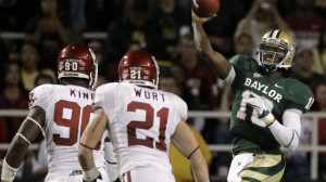
The Chiefs play the Baylor game on an endless loop for the other 31 teams.

The Chiefs play the Baylor game on an endless loop for the other 31 teams.

A few weeks ago, I discovered cfbstats.com, which has made available for download an incredible amount of college football statistics from the last eight seasons. Thanks to them, I plan to apply some of the same techniques I’ve used on NFL numbers over the years to college statistics. If you’re a fan of college football, you’re probably already reading talented writers like Bill Connelly and Brian Fremeau, but hopefully I can bring something new to the table for you to enjoy.

There are many differences between college and professional football, but many of the same stats still matter. For quarterbacks, Adjusted Net Yards per Attempt is still the king of the basic stats [1]For the uninitiated, ANY/A is calculated by starting with passing yards per attempt, adding 20 yards for each touchdown and subtracting 45 yards for each interception, and subtracting sack yards lost … Continue reading, and it is arguably even more important in college where teams play at varying different paces.

There’s a small problem, however, if you want to calculate ANY/A at the college level: the NCAA counts sacks as rush attempts and sack yards lost as negative rushing yards. I manually overrode [2]Unfortunately, some estimation was involved. The player game logs at cfbstats do not identify quarterback sacks, but the team game logs do. So for each quarterback, we know how many passes he threw … Continue reading that decision in my data set, so going forward, all rushing and passing data will include sack data in the preferred manner (keep this in mind when you compare the statistics I present to the “official” ones).
[continue reading…]

References

References
1 For the uninitiated, ANY/A is calculated by starting with passing yards per attempt, adding 20 yards for each touchdown and subtracting 45 yards for each interception, and subtracting sack yards lost from the numerator and adding sacks to the denominator.
2 Unfortunately, some estimation was involved. The player game logs at cfbstats do not identify quarterback sacks, but the team game logs do. So for each quarterback, we know how many passes he threw in the game and how many times his team was sacked. For quarterbacks who threw 100% of their team’s passes in a game, this is easy. However, for quarterbacks who threw fewer than 100% of their team’s passes, they were assigned a pro-rata number of their team’s sacks.
{ 10 comments }

Russell Wilson is too awesome for snide comments.

Russell Wilson is too awesome for snide comments.

Since 1990, there have been 48 rookie quarterbacks that threw at least 224 pass attempts, the necessary amount to qualify for the league’s efficiency ratings. There are many conventional ways to measure rookie quarterbacks, but the off-season lets us play around with more obscure measures.

For example, have you ever considered how rookie quarterbacks performed compared to how their teams passed in the prior year? David Carr, Tim Couch, and Kerry Collins took over expansion teams, but we can compare the passing stats of the other 45 rookie quarterbacks to the team stats from the prior season. To compare across eras, I am grading each individual and team relative to the league average each season.

Let’s start with Net Yards per Attempt. Ben Roethlisberger averaged 7.41 NY/A in 2004 when the league average was 6.14; therefore, Roethlisberger was at 121% of league average. Meanwhile, the 2003 Steelers under Tommy Maddox were at 99% of league average. For each of the 45 rookie quarterbacks, I plotted them in the graph below. The Y-axis shows how the quarterback performed as a rookie, while the X-axis shows how his team performed in the prior season. Because it makes sense to think of “up and to the right” as positive, the X-axis goes in reverse order. Take a look – I have an abbreviation for each quarterback next to his data point:
[continue reading…]

{ 2 comments }

On Monday, I explained my methodology for ranking every wide receiver in football history, and yesterday, I presented a list of the best single seasons of all time. Today the career list of the top 150 wide receivers. As usual, I implemented a 100/95/90 formula, giving a player credit for 100% of his production in his best season, 95% of his value in his second-best season, 90% in his third year, and so on. The table below is fully sortable and lists the first and last year each person played wide receiver [1]Note that I have excluded seasons where a wide receiver played running back or tight end. This is generally not a big deal, but does hurt someone like Lenny Moore.; you can use the search feature to find the best receiver to ever play for each team (for example, typing ‘ram’ for the Rams ‘clt’ for the Colts.)
[continue reading…]

References

References
1 Note that I have excluded seasons where a wide receiver played running back or tight end. This is generally not a big deal, but does hurt someone like Lenny Moore.
{ 55 comments }

Yesterday, I explained my methodology for ranking every wide receiver in football history. Today I’m going to present a list of single-season leaders, which presents some problems.

I think the method I described yesterday does a good job adjusting for era, as receivers are only given credit for their yards above the baseline, which is different each season. But there are some other complicating factors unique to football. Seasons have had varying lengths: a receiver who plays 12 games in a 12-game season can’t be penalized the way you would penalize a receiver who only plays in 12 games now. Since older receivers are generally at a disadvantage for many reasons, I decided to simply pro-rate the value for all non-16 game seasons as if it was a 16-game season. However, I have also included downward adjustments for players in other leagues and during World War II. [1]The fine print: For players in 1943, 1944, and 1945, and for players in the AAFC, I only gave the receivers credit for 60% of the value they created. For the AFL, I gave players 60% of their value in … Continue reading

The table below lists the top 200 wide receiver seasons of all-time.
[continue reading…]

References

References
1 The fine print: For players in 1943, 1944, and 1945, and for players in the AAFC, I only gave the receivers credit for 60% of the value they created. For the AFL, I gave players 60% of their value in 1960 and 1961, 70% in 1962, 80% in 1963, 90% in 1964, and 100% in 1965 through 1969. In case it wasn’t obvious, all of these adjustments are arbitrary.
{ 12 comments }
Next Posts Previous Posts